
 Submit Manuscript
 Peer Review
 Editor Work
- Home
- Articles & Issues
-
Data
- Dataset of Radar Detecting Sea
- SAR Dataset
- SARGroundObjectsTypes
- SARMV3D
- AIRSAT Constellation SAR Land Cover Classification Dataset
- 3DRIED
- UWB-HA4D
- LLS-LFMCWR
- FAIR-CSAR
- MSAR
- SDD-SAR
- FUSAR
- SpaceborneSAR3Dimaging
- Sea-land Segmentation
- SAR Multi-domain Ship Detection Dataset
- SAR-Airport
- Hilly and mountainous farmland time-series SAR and ground quadrat dataset
- SAR images for interference detection and suppression
- HP-SAR Evaluation & Analytical Dataset
- GDHuiYan-ATRNet
- Multi-System Maritime Low Observable Target Dataset
- DatasetinthePaper
- DatasetintheCompetition
- Report
- Course
- About
- Publish
- Editorial Board
- Chinese

| Citation: | Li Hang, Liang Xingdong, Zhang Fubo, Wu Yirong. 3D Imaging for Array InSAR Based on Gaussian Mixture Model Clustering[J]. Journal of Radars, 2017, 6(6): 630-639. doi: 10.12000/JR17020

|
3D Imaging for Array InSAR Based on Gaussian Mixture Model Clustering
DOI: 10.12000/JR17020 CSTR: 32380.14.JR17020
-
Abstract
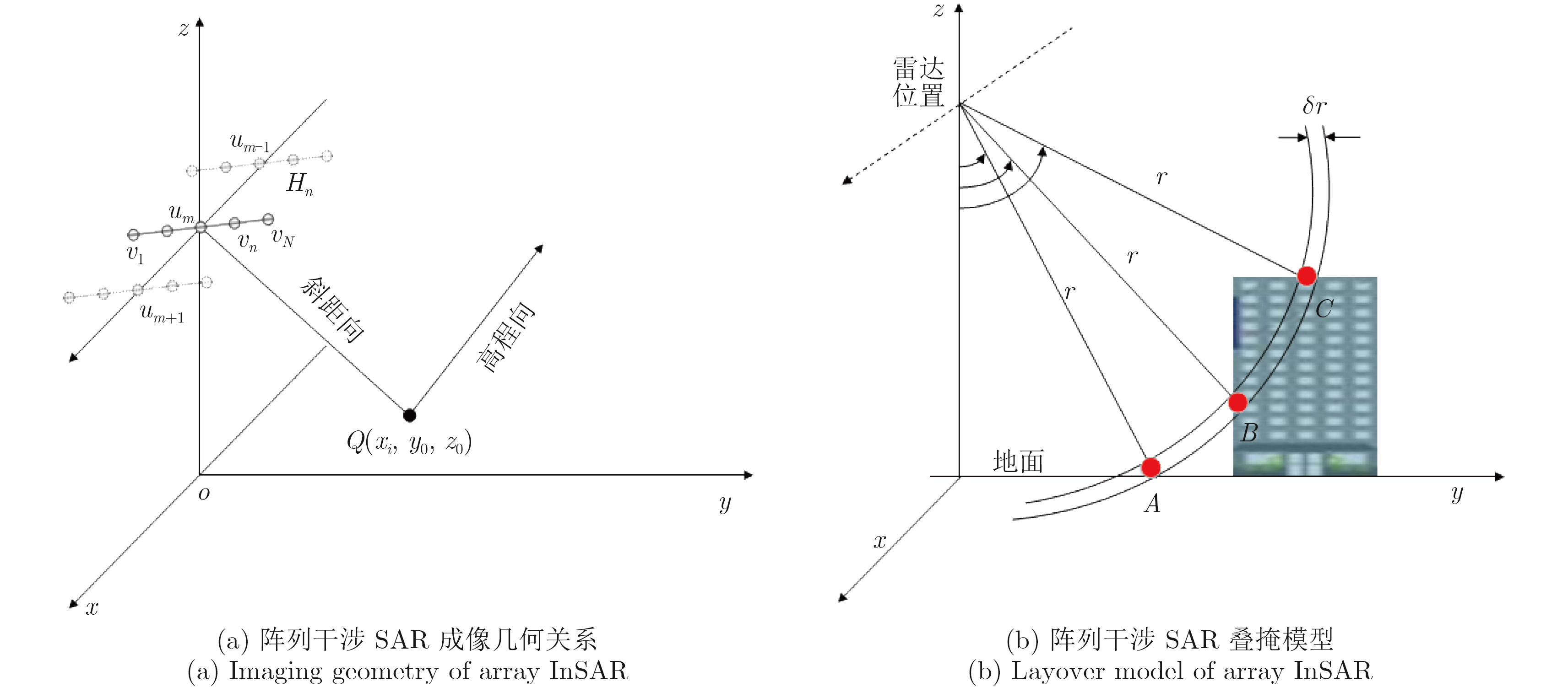
Array InSAR can generate 3D point clouds with the use of SAR images of the observed scene, which are obtained using multiple channels in a single flight. Its resolution power in elevation enables one to solve the layover problem. However, due to the limited number of arrays and the short baseline length, the resolution power in elevation is restricted. Together with the layover phenomenon of the urban buildings, the result of 3D reconstruction suffers from poor accuracy in positioning, and it is difficult to extract the effective characteristics of the buildings. In view of this situation, this paper proposed a 3D reconstruction method of array InSAR based on Gaussian mixture model clustering. First, the 3D point clouds of the observed scene are obtained by an algorithm with super-resolution based on compressive sensing, and then the scatters of buildings are extracted by density estimation; after which the method of Gaussian mixture model clustering is used to classify the 3D point clouds of the buildings. Finally, the inverse SAR images of each region are obtained by using the system parameters, and the 3D reconstruction of the buildings is completed. Based on the actual data of the first domestic 3D imaging experiment by airborne array InSAR, the validity of the algorithm is confirmed and the 3D imaging results of the buildings are obtained.
-

-
References
[1] Morishita Y and Hanssen R F. Temporal decorrelation in L-, C-, and X-band satellite radar interferometry for pasture on drained peat soils[J]. IEEE Transactions on Geoscience and Remote Sensing, 2015, 53(2): 1096–1104. DOI: 10.1109/TGRS.2014.2333814.[2] 张福博. 阵列干涉SAR三维重建信号处理技术研究[D]. [博士论文], 中国科学院大学, 2015.Zhang Fubo. Research on signal processing of 3-D reconstruction in linear array Synthetic Aperture Radar interferometry[D]. [Ph.D.dissertation], Institute of Electronics, Chinese Acedamy of Science, 2015.[3] Knaell K K and Cardillo G P. Radar tomography for the generation of three-dimensional images[J]. IEE Proceedings-Radar, Sonar and Navigation, 1995, 142(2): 54–60. DOI: 10.1049/ip-rsn:19951791.[4] Wang Bin, Wang Yanping, Hong Wen, et al.. Application of spatial spectrum estimation technique in multibaseline SAR for layover solution[C]. Proceedings of IEEE International Geoscience and Remote Sensing Symposium, Boston, USA, 2008: III-1139–III-1142.[5] 王爱春, 向茂生. 基于块压缩感知的SAR层析成像方法[J]. 雷达学报, 2016, 5(1): 57–64. DOI: 10.12000/JR16006.Wang Aichun and Xiang Maosheng. SAR tomography based on block compressive sensing[J]. Journal of Radars, 2016, 5(1): 57–64. DOI: 10.12000/JR16006.[6] Reigber A and Moreira A. First demonstration of airborne SAR tomography using multibaseline L-band data[J]. IEEE Transactions on Geoscience and Remote Sensing, 2000, 38(5): 2142–2152. DOI: 10.1109/36.868873.[7] Zhu Xiaoxiang and Bamler R. Tomographic SAR inversion by L1-norm regularization—the compressive sensing approach[J]. IEEE Transactions on Geoscience and Remote Sensing, 2010, 48(10): 3839–3846. DOI: 10.1109/TGRS.2010.2048117.[8] Zhu Xiaoxiang and Bamler R. Super-resolution power and robustness of compressive sensing for spectral estimation with application to spaceborne tomographic SAR[J]. IEEE Transactions on Geoscience and Remote Sensing, 2012, 50(1): 247–258. DOI: 10.1109/TGRS.2011.2160183.[9] Zivkovic Z. Improved adaptive Gaussian mixture model for background subtraction[C]. Proceedings of the 17th International Conference on Pattern Recognition, Cambridge, UK, 2004, 2: 28–31.[10] Budillon A, Evangelista A, and Schirinzi G. Three-dimensional SAR focusing from multipass signals using compressive sampling[J]. IEEE Transactions on Geoscience and Remote Sensing, 2011, 49(1): 488–499. DOI: 10.1109/TGRS.2010.2054099.[11] Donoho D L. Compressed sensing[J]. IEEE Transactions on Information Theory, 2006, 52(4): 1289–1306. DOI: 10.1109/TIT.2006.871582.[12] 张福博, 梁兴东, 吴一戎. 一种基于地形驻点分割的多通道SAR三维重建方法[J]. 电子与信息学报, 2015, 37(10): 2287–2293. DOI: 10.11999/JEIT150244.Zhang Fu-bo, Liang Xing-dong, and Wu Yi-rong. 3-D reconstruction for multi-channel SAR interferometry using terrain stagnation point based division[J]. Journal of Electronics &Information Technology, 2015, 37(10): 2287–2293. DOI: 10.11999/JEIT150244.[13] 廖明生, 魏恋欢, 汪紫芸, 等. 压缩感知在城区高分辨率SAR层析成像中的应用[J]. 雷达学报, 2015, 4(2): 123–129. DOI: 10.12000/JR15031.Liao Ming-sheng, Wei Lian-huan, Wang Zi-yun, et al. Compressive sensing in high-resolution 3D SAR tomography of urban scenarios[J]. Journal of Radars, 2015, 4(2): 123–129. DOI: 10.12000/JR15031.[14] Zhu Xiaoxiang and Shahzad M. Facade reconstruction using multiview spaceborne TomoSAR point clouds[J]. IEEE Transactions on Geoscience and Remote Sensing, 2014, 52(6): 3541–3552. DOI: 10.1109/TGRS.2013.2273619.[15] Sithole G and Vosselman G. Experimental comparison of filter algorithms for bare-Earth extraction from airborne laser scanning point clouds[J]. ISPRS Journal of Photogrammetry and Remote Sensing, 2004, 59(1-2): 85–101. DOI: 10.1016/j.isprsjprs.2004.05.004.[16] Vosselman G. Slope based filtering of laser altimetry data[J]. International Archives of Photogrammetry and Remote Sensing, 2000, 33(B3/2), Part 3: 935–942.[17] Rottensteiner F and Briese C. A new method for building extraction in urban areas from high-resolution LIDAR data[J]. International Archives of Photogrammetry Remote Sensing and Spatial Information Sciences, 2002, 34(3/A): 295–301.[18] Vrieze S I. Model selection and psychological theory: A discussion of the differences between the Akaike information criterion (AIC) and the Bayesian information criterion (BIC)[J]. Psychological Methods, 2012, 17(2): 228–243. DOI: 10.1037/a0027127.[19] Moon T K. The expectation-maximization algorithm[J]. IEEE Signal Processing Magazine, 1996, 13(6): 47–60. DOI: 10.1109/79.543975.[20] Sampath A and Shan Jie. Segmentation and reconstruction of polyhedral building roofs from aerial lidar point clouds[J]. IEEE Transactions on Geoscience and Remote Sensing, 2010, 48(3): 1554–1567. DOI: 10.1109/TGRS.2009.2030180. -
Proportional views

- Publishing Ethics
- Journal Insights
- Abstracting & Indexing
- Peer Review Policies
- Guide for Authors
- Conference
- ISSN 2095-283X (Print)ISSN 2097-339X (Online)
- CN 10-1030/TN
- CODEN LXEUAO
About Journal
- Sponsor: China Radio Detection and Ranging Industry Association (CRIA)
- Phone: 010-58887062
- Email:radars@aircas.ac.cn
- Publisher: Leida Xuebao Bianjibu (Editorial office of the Journal of Radars)
Contacts Us

京ICP备20021838号-14
Supported by: Beijing Renhe Information Technology Co. Ltd

Export File
Citation
Format
Content
 DownLoad:


- Figure 1. Array InSAR imaging model
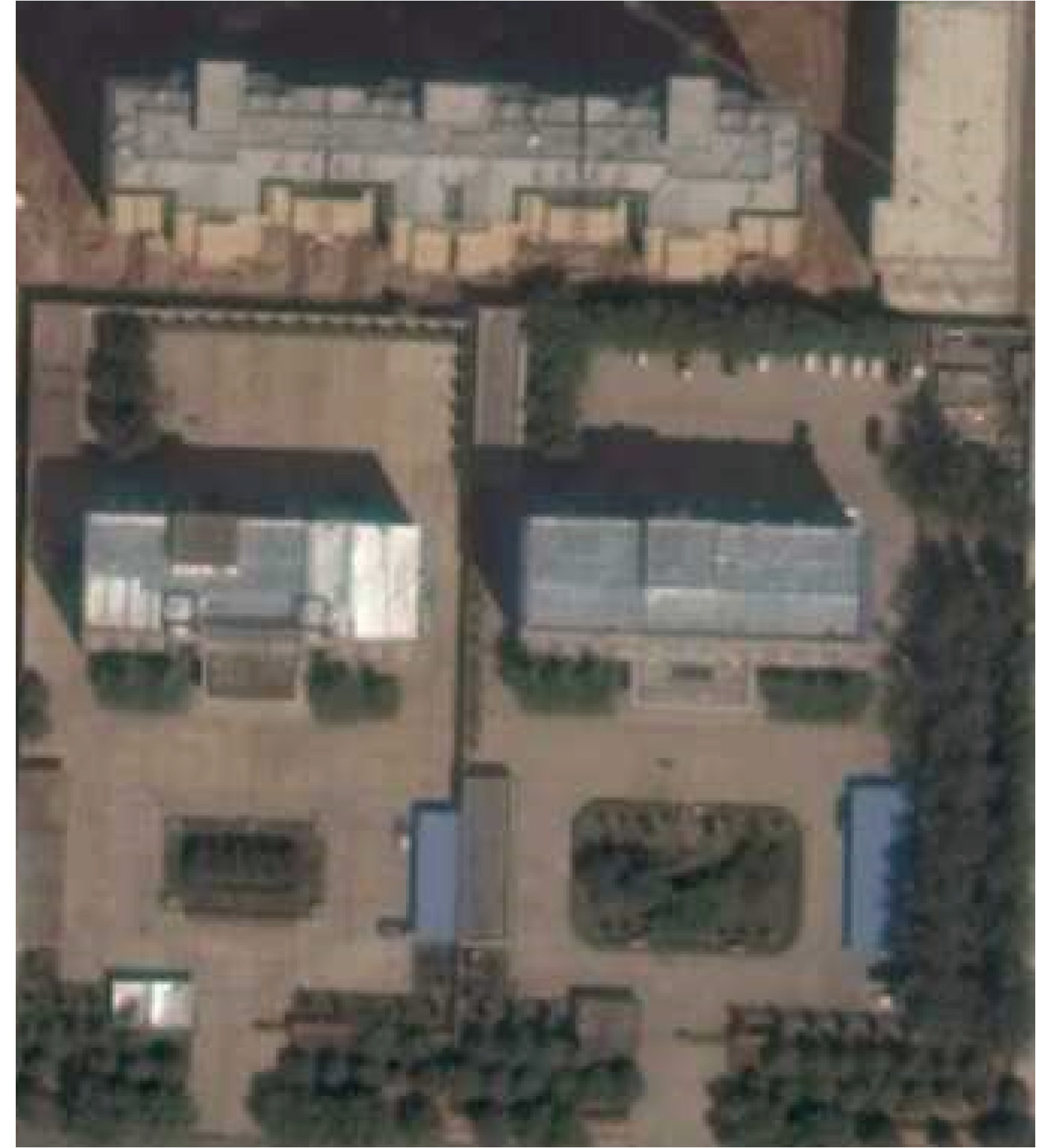
- Figure 2. Optical image of the observed scene
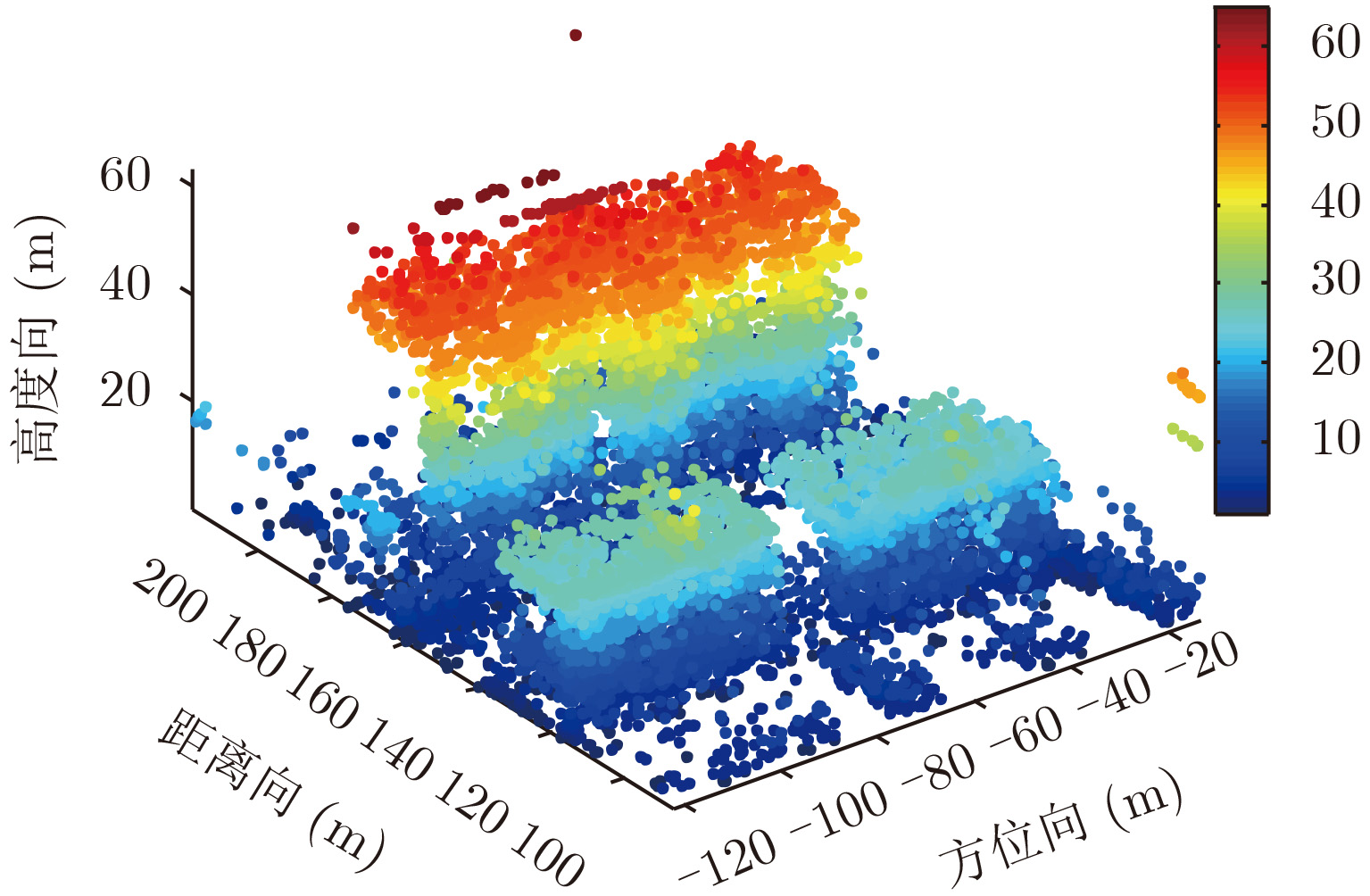
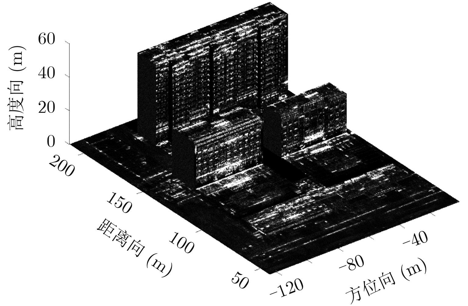
- Figure 3. Orginal 3D point clouds of the observed scene
- Figure 4. Workflow of proposed approach
- Figure 5. Scatterer density map of the observed scene
- Figure 6. Extracted building results of the observed scene
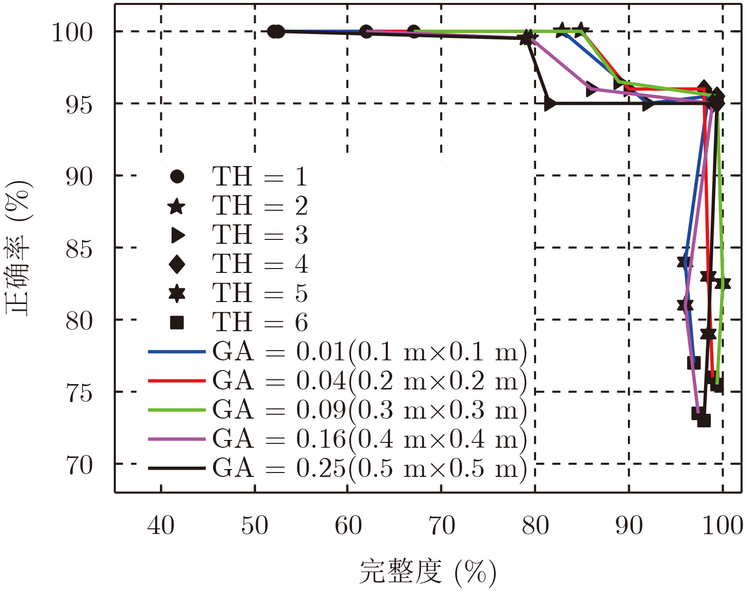
- Figure 7. Performance curve map with varying TH and GA parameters
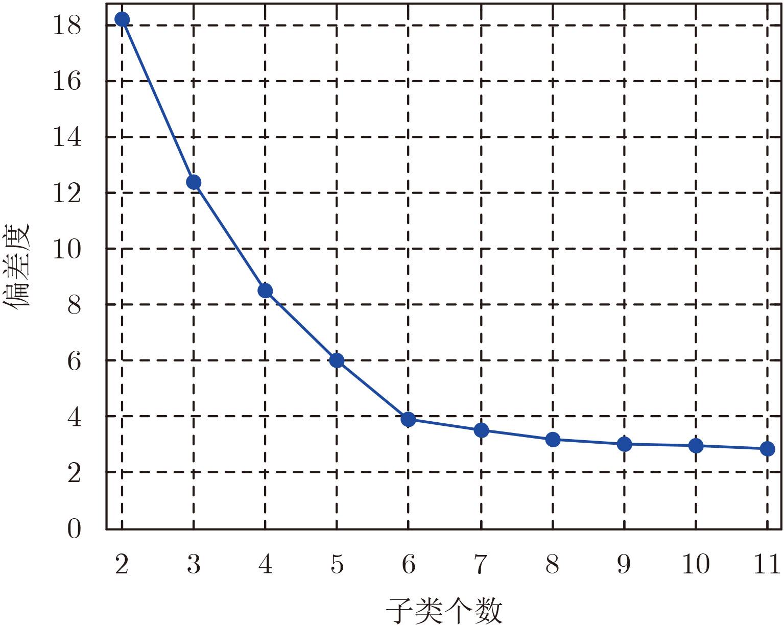
- Figure 8. Dispersion plot with number of clusters
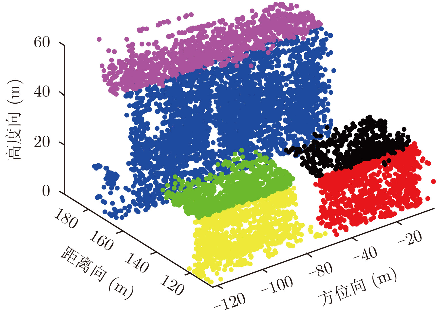
- Figure 9. Clustered result of building areas
- Figure 10. Clustered results of K-means
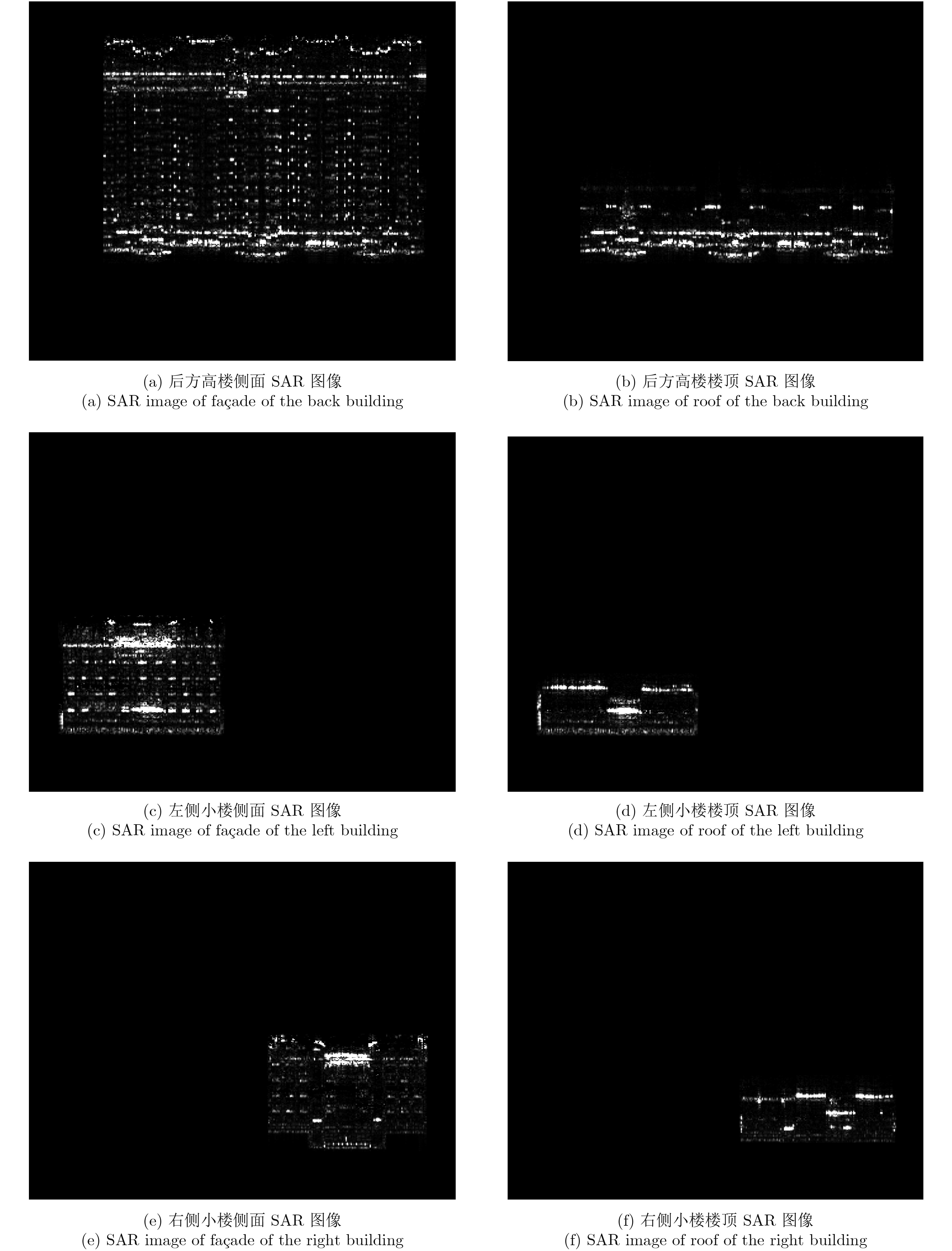
- Figure 11. Inversed SAR images of all aeras
- Figure 12. Inversed SAR images of the ground
- Figure 13. 2D SAR image of the observed scene
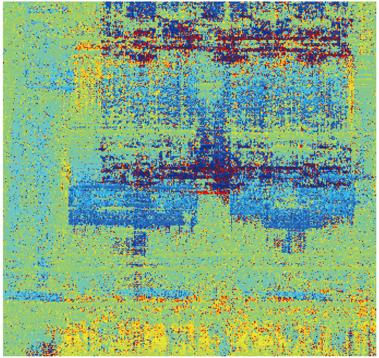
- Figure 14. Interferometric phase image of the observed scene
- Figure 15. 3D imaging result of the observed scene