
 Submit Manuscript
 Peer Review
 Editor Work
- Home
- Articles & Issues
-
Data
- Dataset of Radar Detecting Sea
- SAR Dataset
- SARGroundObjectsTypes
- SARMV3D
- AIRSAT Constellation SAR Land Cover Classification Dataset
- 3DRIED
- UWB-HA4D
- LLS-LFMCWR
- FAIR-CSAR
- MSAR
- SDD-SAR
- FUSAR
- SpaceborneSAR3Dimaging
- Sea-land Segmentation
- SAR Multi-domain Ship Detection Dataset
- SAR-Airport
- Hilly and mountainous farmland time-series SAR and ground quadrat dataset
- SAR images for interference detection and suppression
- HP-SAR Evaluation & Analytical Dataset
- GDHuiYan-ATRNet
- Multi-System Maritime Low Observable Target Dataset
- DatasetinthePaper
- DatasetintheCompetition
- Report
- Course
- About
- Publish
- Editorial Board
- Chinese
| Citation: | YIN Junjun, LUO Jiahao, LI Xiang, et al. Ship detection based on polarimetric SAR gradient and complex Wishart classifier[J]. Journal of Radars, 2024, 13(2): 396–397. doi: 10.12000/JR23198

|
Ship Detection Based on Polarimetric SAR Gradient and Complex Wishart Classifier
DOI: 10.12000/JR23198 CSTR: 32380.14.JR23198
More Information-
Abstract
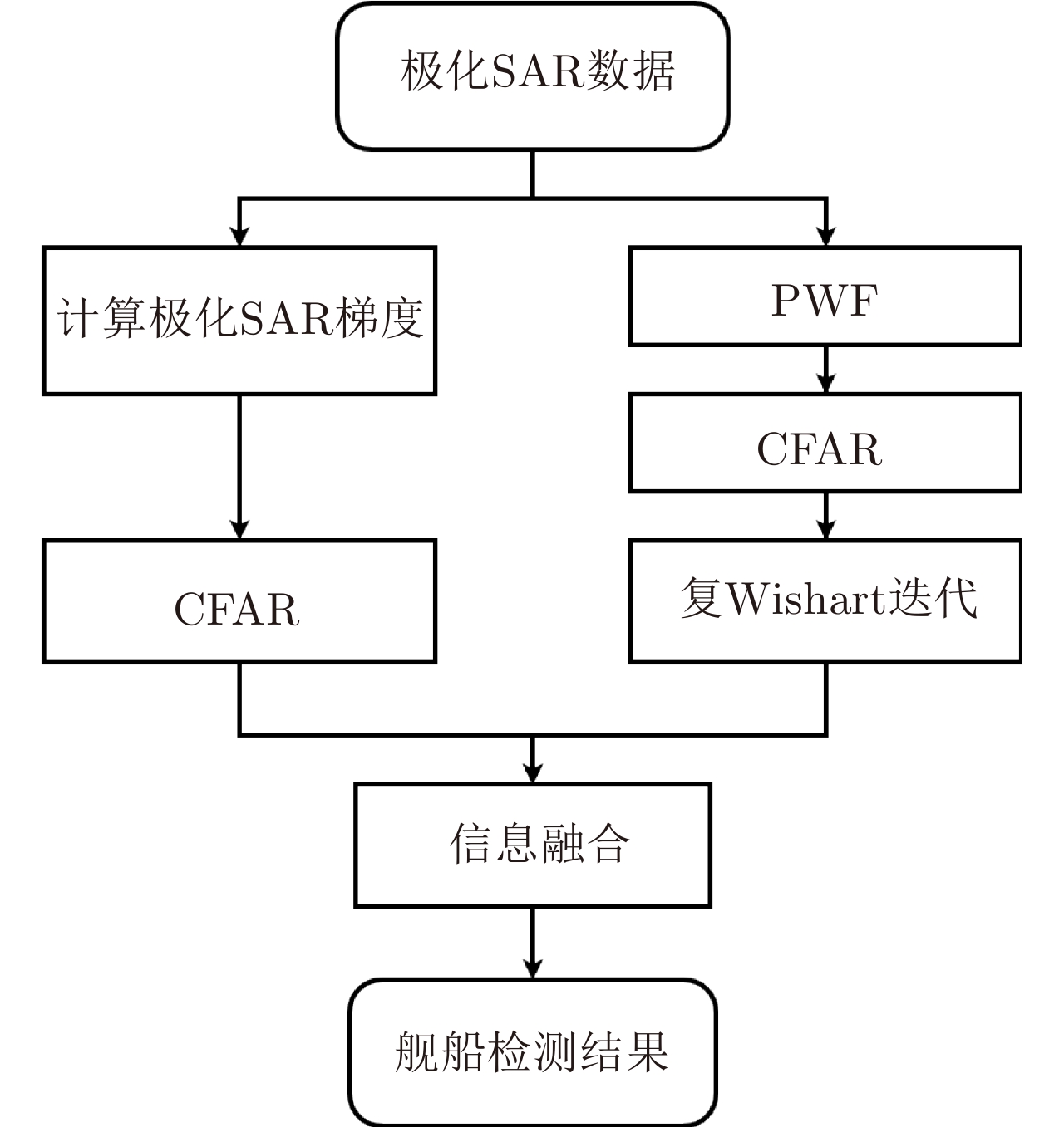
Ship detection is one of the most important applications of polarimetric Synthetic Aperture Radar (SAR) systems. Current ship detection methods are susceptible to side flap interference, making it difficult to extract the target shape correctly. In addition, when ships are exceedingly dense and have different scales, adjacent ships may be considered as a single target because of the influence of strong sidelobes, causing missed detections. To address the issues of sidelobe interference and multi-scale dense ship detection, a ship detection method based on the polarimetric SAR gradient and the complex Wishart classifier is proposed. First, the Likelihood Ratio Test (LRT) gradient is introduced into the log-ratio gradient framework to apply it to the polarimetric SAR data. Then, a Constant False Alarm Rate (CFAR) detector is applied to the gradient image to map the ship boundaries accurately. Second, the complex Wishart iterative classifier is used to detect the strong scattering part of the ship, which can eliminate most clutter interference and maintain the ship’s shape details. Finally, the LRT detection and complex Wishart classifier detection results are fused. Thus, not only the strong sidelobe interference can be greatly suppressed, but the dense targets with different scales are also distinguished and accurately located. This study performs comparative experiments on three polarimetric SAR images from the ALOS-2 satellite. Experimental results show that compared with the existing methods, the proposed algorithm has fewer false alarms and missed detections and can effectively overcome the problems of sidelobe interference while maintaining the shape details. -

-
References
[1] 杨汝良, 戴博伟, 李海英. 极化合成孔径雷达极化层次和系统工作方式[J]. 雷达学报, 2016, 5(2): 132–142. doi: 10.12000/JR16013.YANG Ruliang, DAI Bowei, and LI Haiying. Polarization hierarchy and system operating architecture for polarimetric synthetic aperture radar[J]. Journal of Radars, 2016, 5(2): 132–142. doi: 10.12000/JR16013.[2] WEISS M. Analysis of some modified cell-averaging CFAR processors in multiple-target situations[J]. IEEE Transactions on Aerospace and Electronic Systems, 1982, AES-18(1): 102–114. doi: 10.1109/TAES.1982.309210.[3] NOVAK L M, BURL M C, and IRVING W W. Optimal polarimetric processing for enhanced target detection[J]. IEEE Transactions on Aerospace and Electronic Systems, 1993, 29(1): 234–244. doi: 10.1109/7.249129.[4] AI Jiaqiu, YANG Xuezhi, DONG Zhangyu, et al. A new two parameter CFAR ship detector in Log-Normal clutter[C]. 2017 IEEE Radar Conference, Seattle, USA, 2017: 195–199. doi: 10.1109/RADAR.2017.7944196.[5] RITCEY J A and DU H. Order statistic CFAR detectors for speckled area targets in SAR[C]. Conference Record of the Twenty-Fifth Asilomar Conference on Signals, Systems & Computers, Pacific Grove, USA, 1991: 1082–1086. doi: 10.1109/ACSSC.1991.186613.[6] GOLDSTEIN G B. False-alarm regulation in log-normal and Weibull clutter[J]. IEEE Transactions on Aerospace and Electronic Systems, 1973, AES-9(1): 84–92. doi: 10.1109/TAES.1973.309705.[7] LEVANON N and SHOR M. Order statistcs CFAR for Weibull background[J]. IEE Proceedings F (Radar and Signal Processing), 1990, 137(3): 157–162. doi: 10.1049/ip-f-2.1990.0023.[8] ANASTASSOPOULOS V and LAMPROPOULOS G A. Optimal CFAR detection in Weibull clutter[J]. IEEE Transactions on Aerospace and Electronic Systems, 1995, 31(1): 52–64. doi: 10.1109/7.366292.[9] GUAN Jian, HE You, and PENG Yingning. CFAR detection in K-distributed clutter[C]. Fourth International Conference on Signal Processing, Beijing, China, 1998: 1513–1516. doi: 10.1109/ICOSP.1998.770911.[10] NOVAK L M and BURL M C. Optimal speckle reduction in polarimetric SAR imagery[J]. IEEE Transactions on Aerospace and Electronic Systems, 1990, 26(2): 293–305. doi: 10.1109/7.53442.[11] 杨汝良, 戴博伟, 谈璐璐, 等. 极化微波成像[M]. 北京: 国防工业出版社, 2016.YANG Ruliang, DAI Bowei, TAN Lulu, et al. Polarimetric Microwave Imaging[M]. Beijing: National Defense Industry Press, 2016.[12] CHANEY R D, BUD M C, and NOVAK L M. On the performance of polarimetric target detection algorithms[J]. IEEE Aerospace and Electronic Systems Magazine, 1990, 5(11): 10–15. doi: 10.1109/62.63157.[13] BOERNER W M, KOSTINSKI A B, and JAMES B D. On the concept of the polarimetric matched filter in high resolution radar imaging: An alternative for speckle reduction[C]. International Geoscience and Remote Sensing Symposium, ‘Remote Sensing: Moving Toward the 21st Century’, Edinburgh, UK, 1988: 69–72. doi: 10.1109/IGARSS.1988.570053.[14] KOSTINSKI A and BOERNER W. On the polarimetric contrast optimization[J]. IEEE Transactions on Antennas and Propagation, 1987, 35(8): 988–991. doi: 10.1109/TAP.1987.1144209.[15] YANG Jian, DONG Guiwei, PENG Yingning, et al. Generalized optimization of polarimetric contrast enhancement[J]. IEEE Geoscience and Remote Sensing Letters, 2004, 1(3): 171–174. doi: 10.1109/LGRS.2004.830127.[16] 殷君君, 安文韬, 杨健. 基于极化散射参数与Fisher-OPCE的监督目标分类[J]. 清华大学学报: 自然科学版, 2011, 51(12): 1782–1786. doi: 10.16511/j.cnki.qhdxxb.2011.12.007.YIN Junjun, AN Wentao, and YANG Jian. Supervised target classification using polarimetric scattering parameters and Fisher-OPCE[J]. Journal of Tsinghua University : Science and Technolog y, 2011, 51(12): 1782–1786. doi: 10.16511/j.cnki.qhdxxb.2011.12.007.[17] XI Yuyang, ZHANG Xi, LAI Quan, et al. A new PolSAR ship detection metric fused by polarimetric similarity and the third eigenvalue of the coherency matrix[C]. 2016 IEEE International Geoscience and Remote Sensing Symposium, Beijing, China, 2016: 112–115. doi: 10.1109/IGARSS.2016.7729019.[18] ZHANG Tao, YANG Zhen, and XIONG Huilin. PolSAR ship detection based on the polarimetric covariance difference matrix[J]. IEEE Journal of Selected Topics in Applied Earth Observations and Remote Sensing, 2017, 10(7): 3348–3359. doi: 10.1109/JSTARS.2017.2671904.[19] SHI Hao, ZHANG Qingjun, BIAN Mingming, et al. A novel ship detection method based on gradient and integral feature for single-polarization synthetic aperture radar imagery[J]. Sensors, 2018, 18(2): 563. doi: 10.3390/s18020 563.[20] DELLINGER F, DELON J, GOUSSEAU Y, et al. SAR-SIFT: A SIFT-like algorithm for SAR images[J]. IEEE Transactions on Geoscience and Remote Sensing, 2015, 53(1): 453–466. doi: 10.1109/TGRS.2014.2323552.[21] SONG Shengli, XU Bin, and YANG Jian. SAR target recognition via supervised discriminative dictionary learning and sparse representation of the SAR-HOG feature[J]. Remote Sensing, 2016, 8(8): 683. doi: 10.3390/rs8080683.[22] LIN Huiping, SONG Shengli, and YANG Jian. Ship classification based on MSHOG feature and task-driven dictionary learning with structured incoherent constraints in SAR images[J]. Remote Sensing, 2018, 10(2): 190. doi: 10.3390/rs10020190.[23] GAO Gui. A parzen-window-kernel-based CFAR algorithm for ship detection in SAR images[J]. IEEE Geoscience and Remote Sensing Letters, 2011, 8(3): 557–561. doi: 10.1109/LGRS.2010.2090492.[24] 张晓玲, 张天文, 师君, 等. 基于深度分离卷积神经网络的高速高精度SAR舰船检测[J]. 雷达学报, 2019, 8(6): 841–851. doi: 10.12000/JR19111.ZHANG Xiaoling, ZHANG Tianwen, SHI Jun, et al. High-speed and high-accurate SAR ship detection based on a depthwise separable convolution neural network[J]. Journal of Radars, 2019, 8(6): 841–851. doi: 10.12000/JR19111.[25] FAN Weiwei, ZHOU Feng, BAI Xueru, et al. Ship detection using deep convolutional neural networks for PolSAR images[J]. Remote Sensing, 2019, 11(23): 2862. doi: 10.3390/rs11232862.[26] AN Quanzhi, PAN Zongxu, and YOU Hongjian. Ship detection in Gaofen-3 SAR images based on sea clutter distribution analysis and deep convolutional neural network[J]. Sensors, 2018, 18(2): 334. doi: 10.3390/s18020334.[27] ZHANG Zhimian, WANG Haipeng, XU Feng, et al. Complex-valued convolutional neural network and its application in polarimetric SAR image classification[J]. IEEE Transactions on Geoscience and Remote Sensing, 2017, 55(12): 7177–7188. doi: 10.1109/TGRS.2017.2743222.[28] RIGNOT E J M and VAN ZYL J J. Change detection techniques for ERS-1 SAR data[J]. IEEE Transactions on Geoscience and Remote Sensing, 1993, 31(4): 896–906. doi: 10.1109/36.239913.[29] MA Xiaoshuang, SHEN Huanfeng, ZHANG Liangpei, et al. Adaptive anisotropic diffusion method for polarimetric SAR speckle filtering[J]. IEEE Journal of Selected Topics in Applied Earth Observations and Remote Sensing, 2015, 8(3): 1041–1050. doi: 10.1109/JSTARS.2014.2328332.[30] NIELSEN A A, CONRADSEN K, and SKRIVER H. Change detection in full and dual polarization, single-and multifrequency SAR data[J]. IEEE Journal of Selected Topics in Applied Earth Observations and Remote Sensing, 2015, 8(8): 4041–4048. doi: 10.1109/JSTARS.2015.2416434.[31] LEE J S, GRUNES M R, AINSWORTH T L, et al. Unsupervised classification using polarimetric decomposition and the complex Wishart classifier[J]. IEEE Transactions on Geoscience and Remote Sensing, 1999, 37(5): 2249–2258. doi: 10.1109/36.789621.[32] 张嘉峰, 朱博, 张鹏, 等. Wishart分布情形下极化SAR图像目标CFAR检测解析方法[J]. 电子学报, 2018, 46(2): 433–439. doi: 10.3969/j.issn.0372-2112.2018.02.024.ZHANG Jiafeng, ZHU Bo, ZHANG Peng, et al. Polarimetric SAR imagery target CFAR detection analytical algorithm with Wishart distribution[J]. Acta Electronica Sinica, 2018, 46(2): 433–439. doi: 10.3969/j.issn.0372-2112.2018.02.024.[33] WANG Hongmiao, ZENG Liang, ZHANG Tao, et al. A PolSAR despeckling method based on Wishart gradient and anisotropic diffusion[J]. Electronics Letters, 2021, 57(3): 126–128. doi: 10.1049/ell2.12086. -
Proportional views

- Publishing Ethics
- Journal Insights
- Abstracting & Indexing
- Peer Review Policies
- Guide for Authors
- Conference
- ISSN 2095-283X (Print)ISSN 2097-339X (Online)
- CN 10-1030/TN
- CODEN LXEUAO
About Journal
- Sponsor: China Radio Detection and Ranging Industry Association (CRIA)
- Phone: 010-58887062
- Email:radars@aircas.ac.cn
- Publisher: Leida Xuebao Bianjibu (Editorial office of the Journal of Radars)
Contacts Us

京ICP备20021838号-14
Supported by: Beijing Renhe Information Technology Co. Ltd

Export File
Citation
Format
Content
 DownLoad:


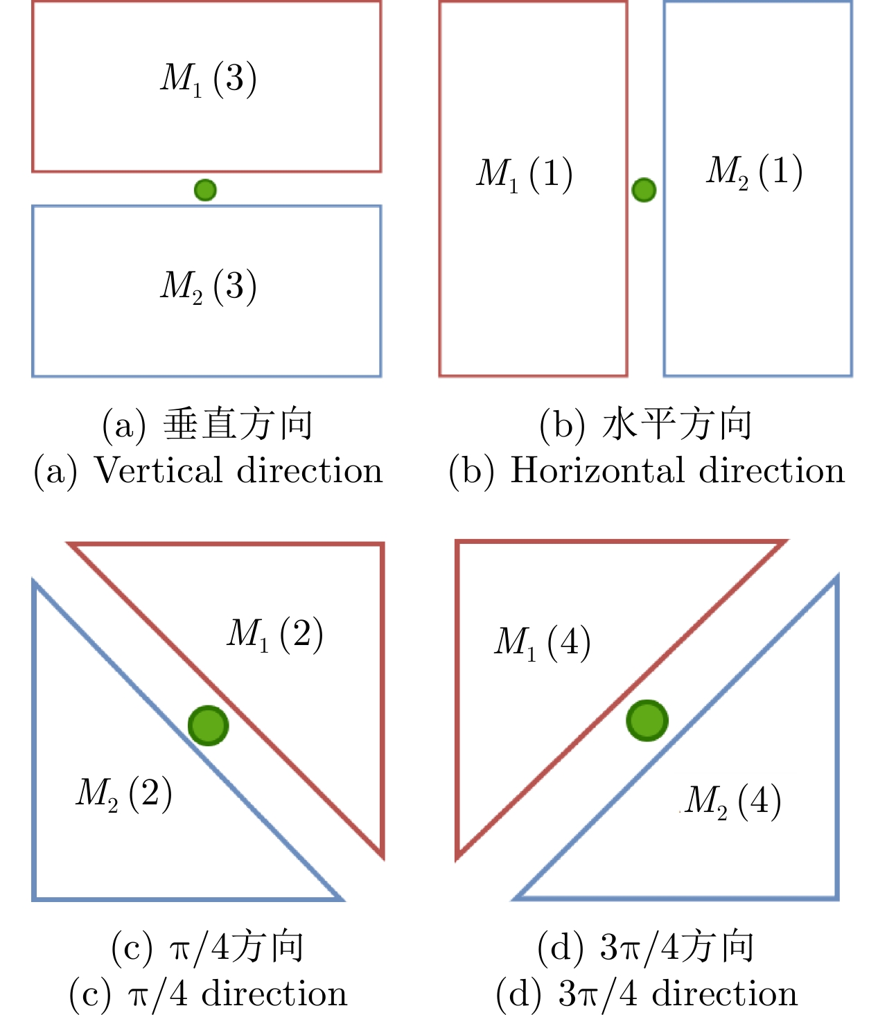
- Figure 1. Scheme of the ROA method
- Figure 2. Flow chart of the proposed method
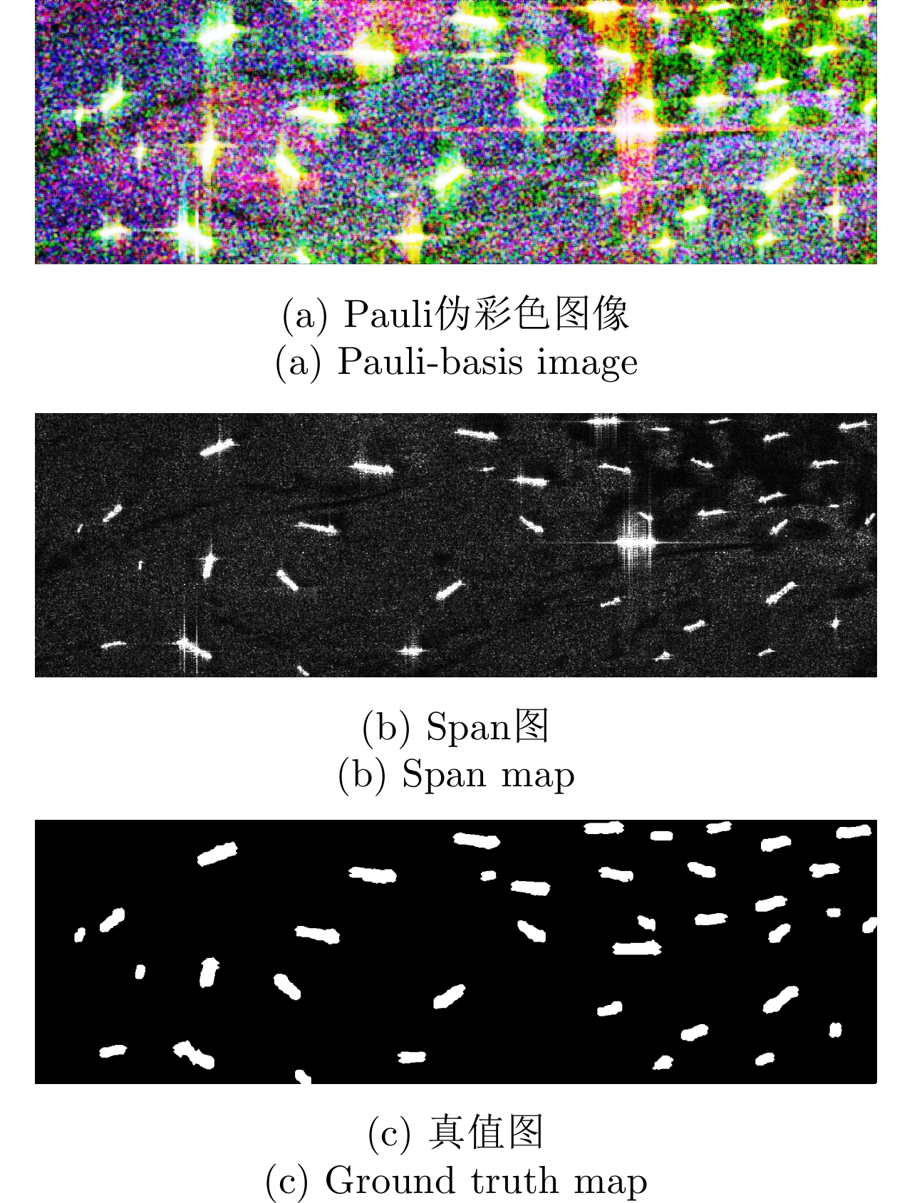
- Figure 3. Experimental scene 1
- Figure 4. Experimental scene 2 (first line) and experimental scene 3 (second line)
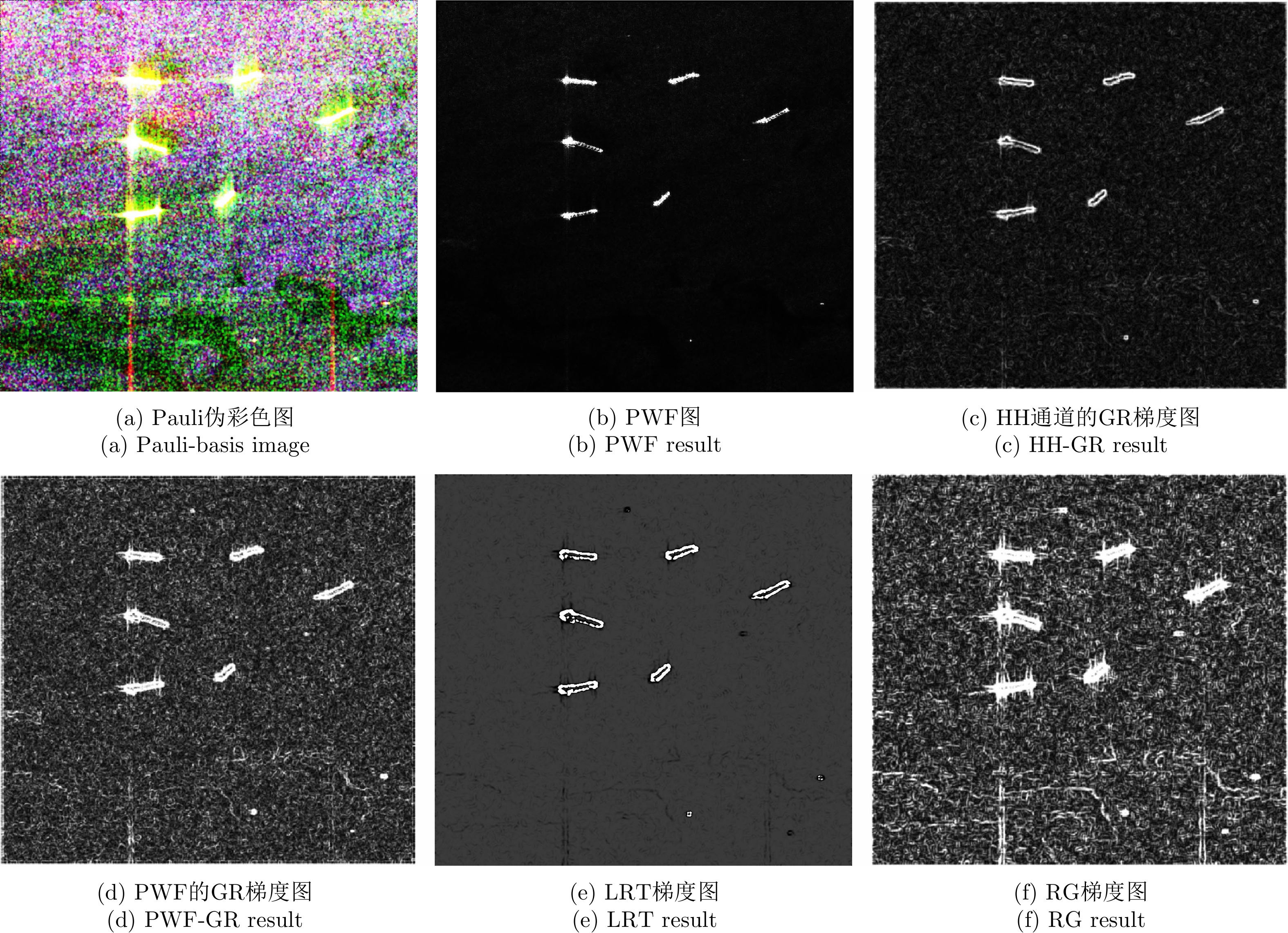
- Figure 5. Calculation results for different gradients
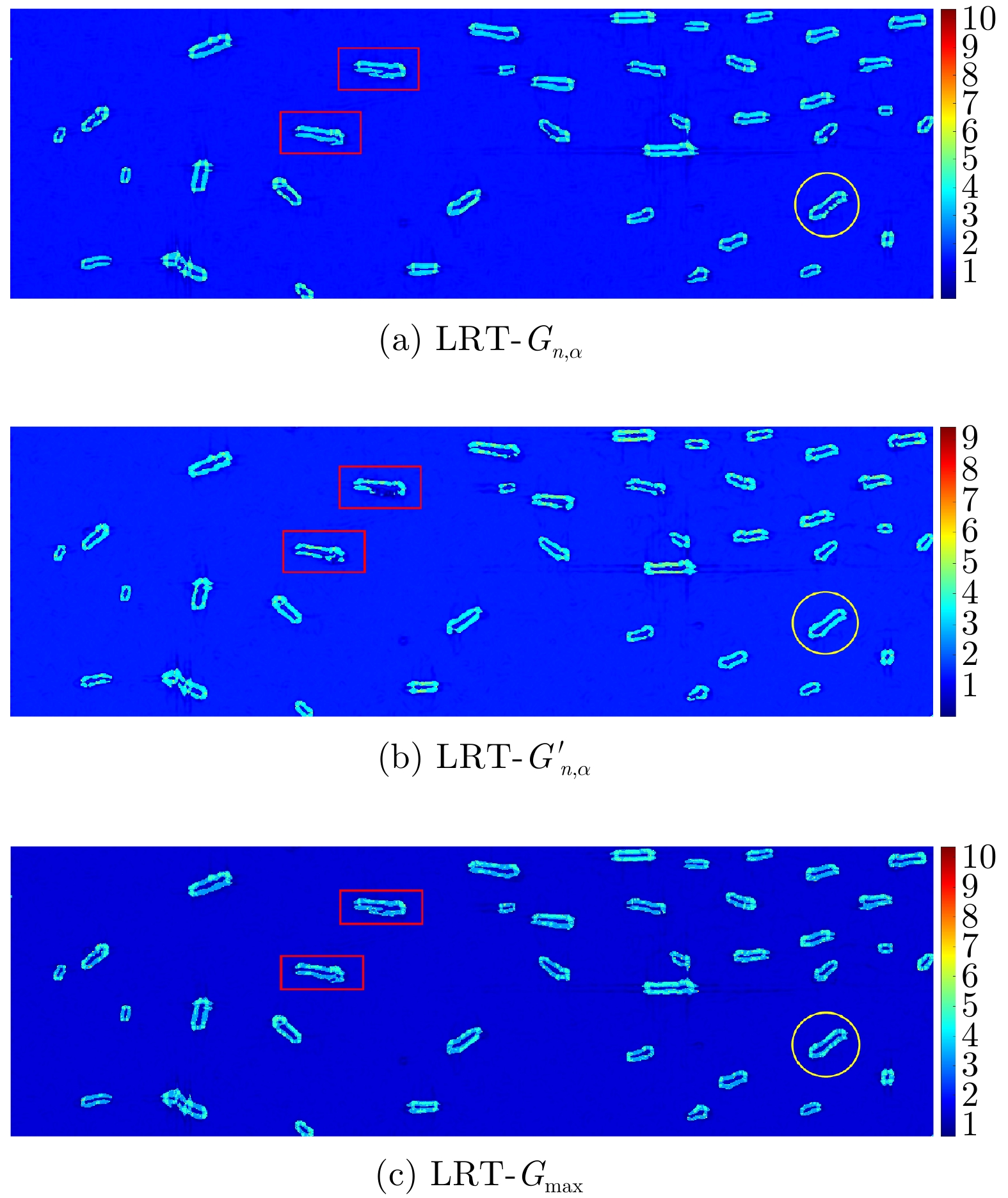
- Figure 6. Comparison of three LRT gradient calculation results
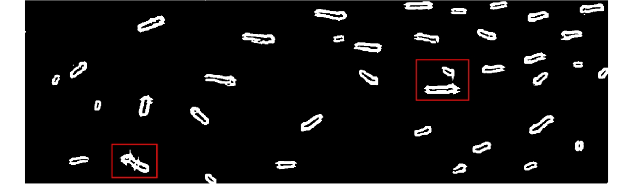
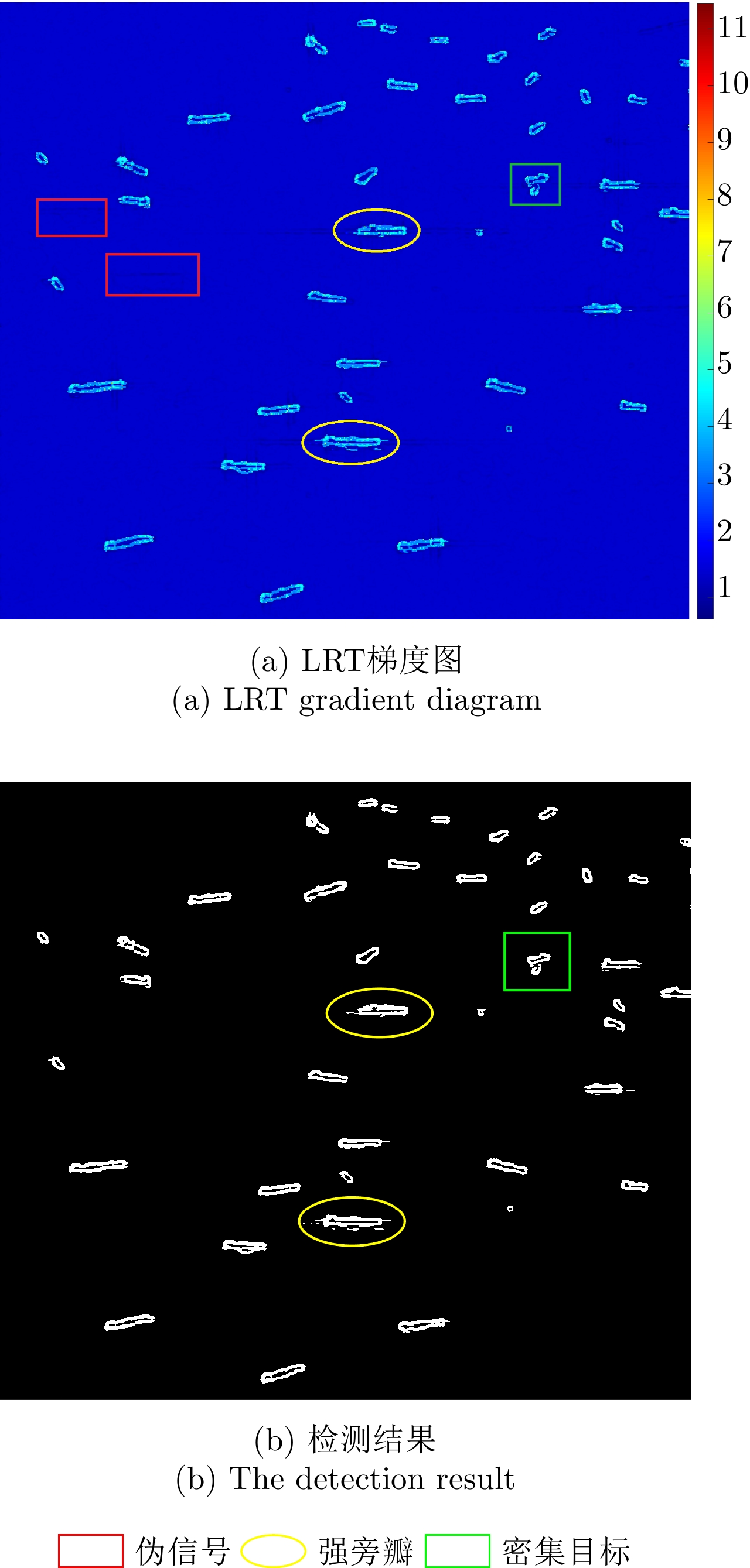
- Figure 7. The detection result of LRT gradient
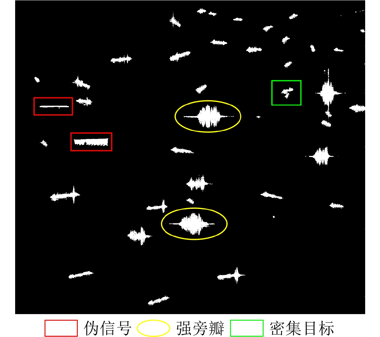
- Figure 8. The detection result of PWF
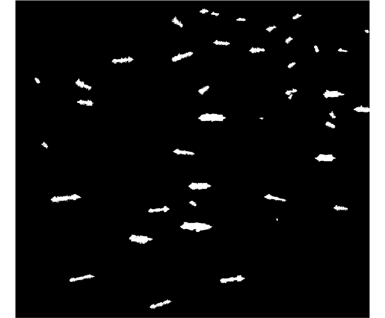
- Figure 9. The classification result of complex Wishart classifier
- Figure 10. Pseudo-color display of the sum of LRT detection result and complex Wishart result
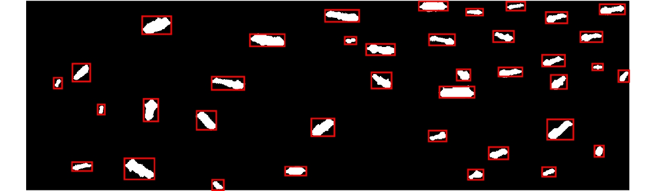
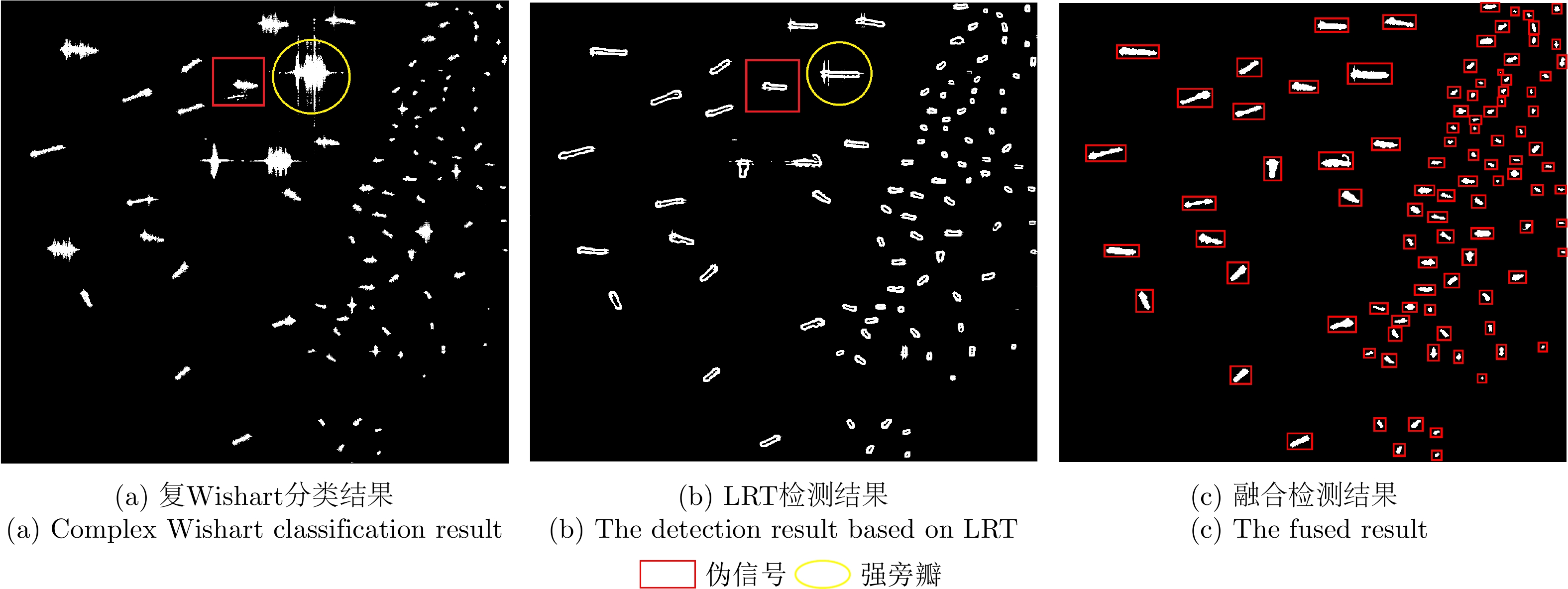
- Figure 11. The fused result
- Figure 12. Image of pseudo-signal and sidelobes
- Figure 13. CFAR detection results based on LRT
- Figure 14. The fused result for complex sea surface scenario
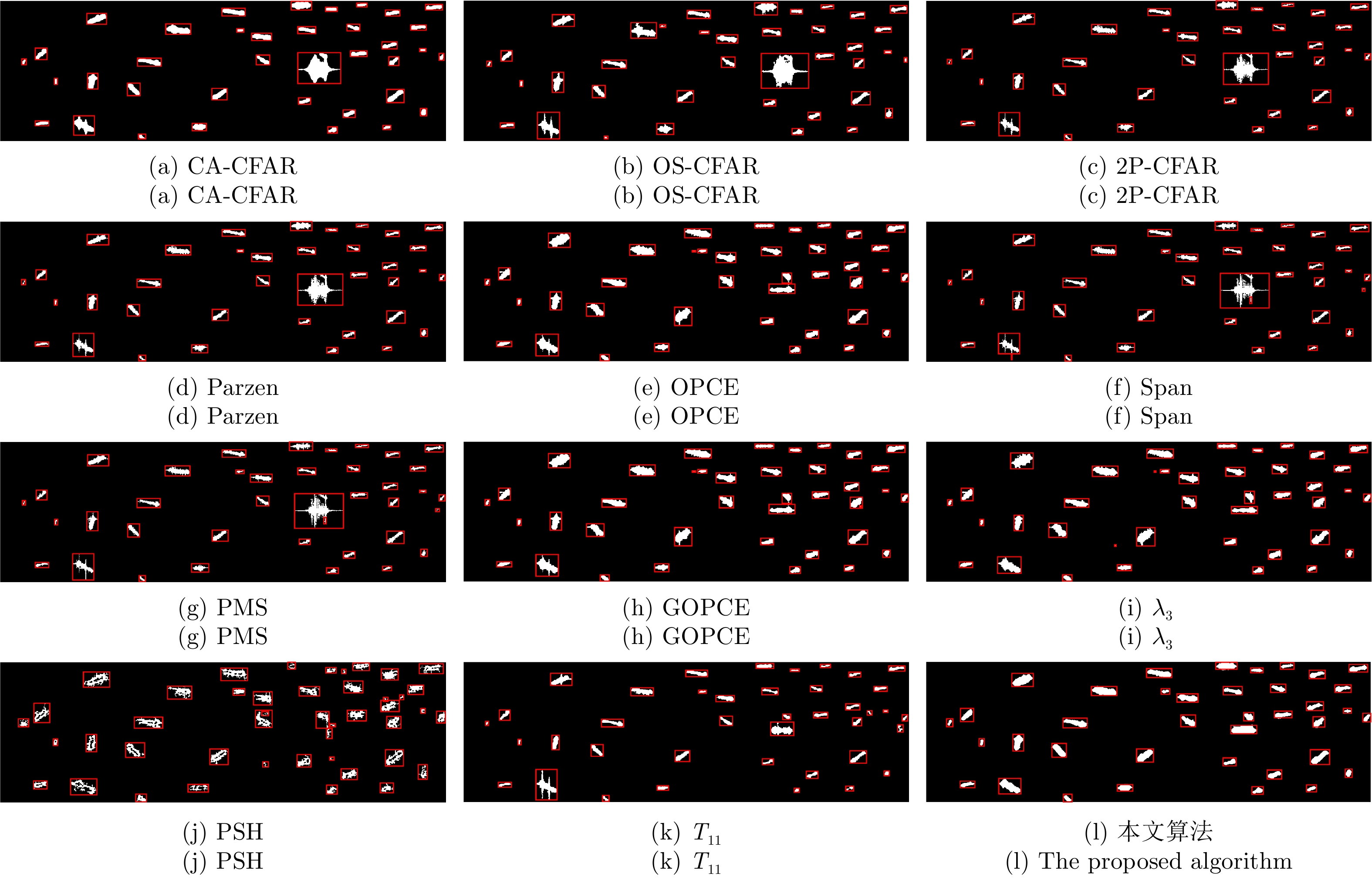
- Figure 15. Multi-scale ship detection results
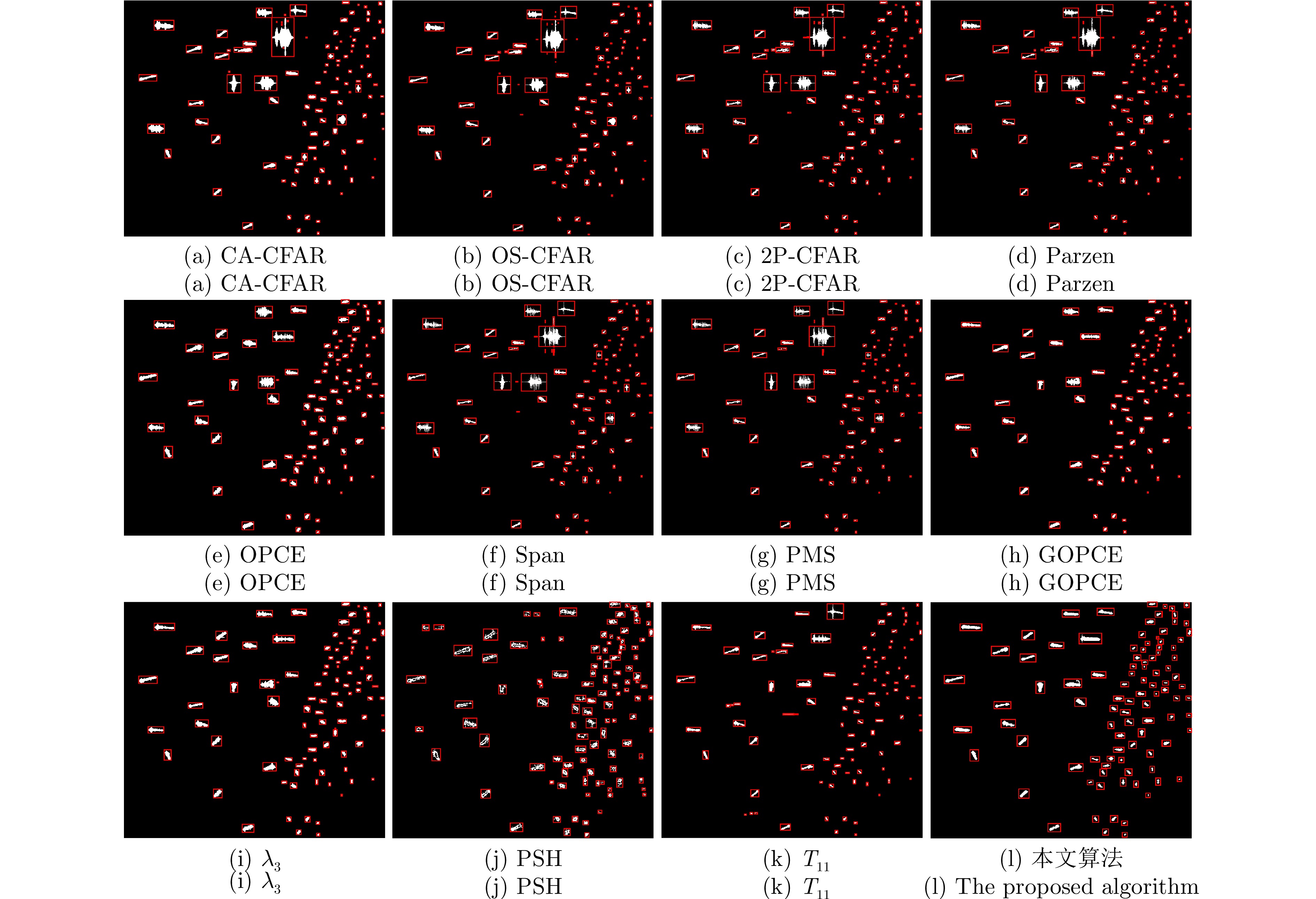
- Figure 16. Ship detection results for experimental scenario 2
- Figure 17. Ship detection results for experimental scenario 3
- Figure 18. Ship detection results for experimental scenario 1