
 作者中心
作者中心 专家审稿
专家审稿 责编办公
责编办公 编辑办公
编辑办公
Performance Investigation on Elevation Cascaded Digital Beamforming for Multidimensional Waveform Encoding SAR Imaging
DOI: 10.12000/JR20107 cstr: 32380.14.JR20107
-
摘要: 在采用多维波形编码(MWE)技术的新体制合成孔径雷达(SAR)系统中,利用俯仰向的数字波束形成(DBF)来实现多个发射波形重叠回波的可靠分离是一个关键问题。该文详细研究了星上实时波束控制与地面后置零陷控制相结合的混合俯仰向DBF分离方法的成像性能问题。 作为一种包括星地两级DBF网络的级联结构,其中的星上部分通过在划分的多个天线子孔径上实现实时主瓣波束指向控制,确保在整个测绘上足够的信号接收增益; 而后置自适应DBF网络主要完成零陷抑制的任务,以消除其它发射波形带来的距离向干扰,可自适应于地形高度起伏变化带来的视角变化。根据对发射波形时频结构先验信息的利用情况,提出了两种星上实时波束形成器的实现方式。对混合DBF方法下的成像信噪比和模糊度性能进行了理论建模与仿真实验评估。实验结果表明,混合DBF方法可以为优化图像模糊度和信噪比性能提供额外的设计自由度,并降低星上数据通道数目。与纯地面DBF网络相比,采用混合DBF网络可以在显著减少星上输出数据量的同时获得满意的性能,在给出的实例中,实现相近性能的条件下,相应的星上数据通道数从10个减少到6个。Abstract: An important issue in a Synthetic Aperture Radar (SAR) system employing Multidimensional Waveform Encoding (MWE) is the fulfillments of Digital BeamForming (DBF) on receive in elevation for a reliable separation of the mutually overlapped echoes from multiple transmit waveforms. In this paper, the performance of a separation approach employing hybrid DBF in elevation by combining the onboard real-time beam-steering and a posteriori null-steering DBF on the ground is elaborately investigated. As a cascaded structure which comprises two subsequent DBF networks, the onboard part effectuates the steering of the mainlobes within multiple partitioned groups of antenna elements to ensure sufficient signal receive gain over the whole swath; the a posteriori adaptive DBF network on the ground mainly performs the task of placing nulls to cancel the range interference from other transmit waveforms, which enables adaptive beamforming to avoid the topographic height variation problem. Two type of onboard realtime beamformers are investigated, depending on the utilization of the transmit waveform structure information or not. The performance of the hybrid DBF approach is theoretically analyzed and evaluated in simulation experiment. It is shown that the hybrid DBF approach can provide additional dimensions of the trade-space to optimize the performance on range ambiguity suppression and signal-to-noise ratio improvement, as well as the onboard data volume reduction. In comparison with the a posteriori DBF on the ground, employing the hybrid DBF networks can get satisfactory performance while remarkably reducing the output data volume, in the presented example, the corresponding output channel number is decreased from 10 to 6.
-
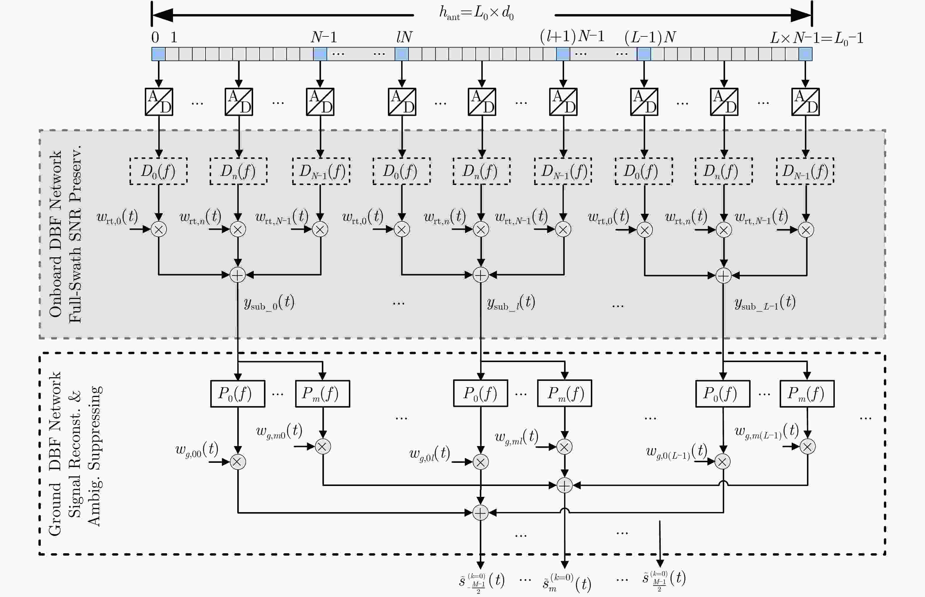
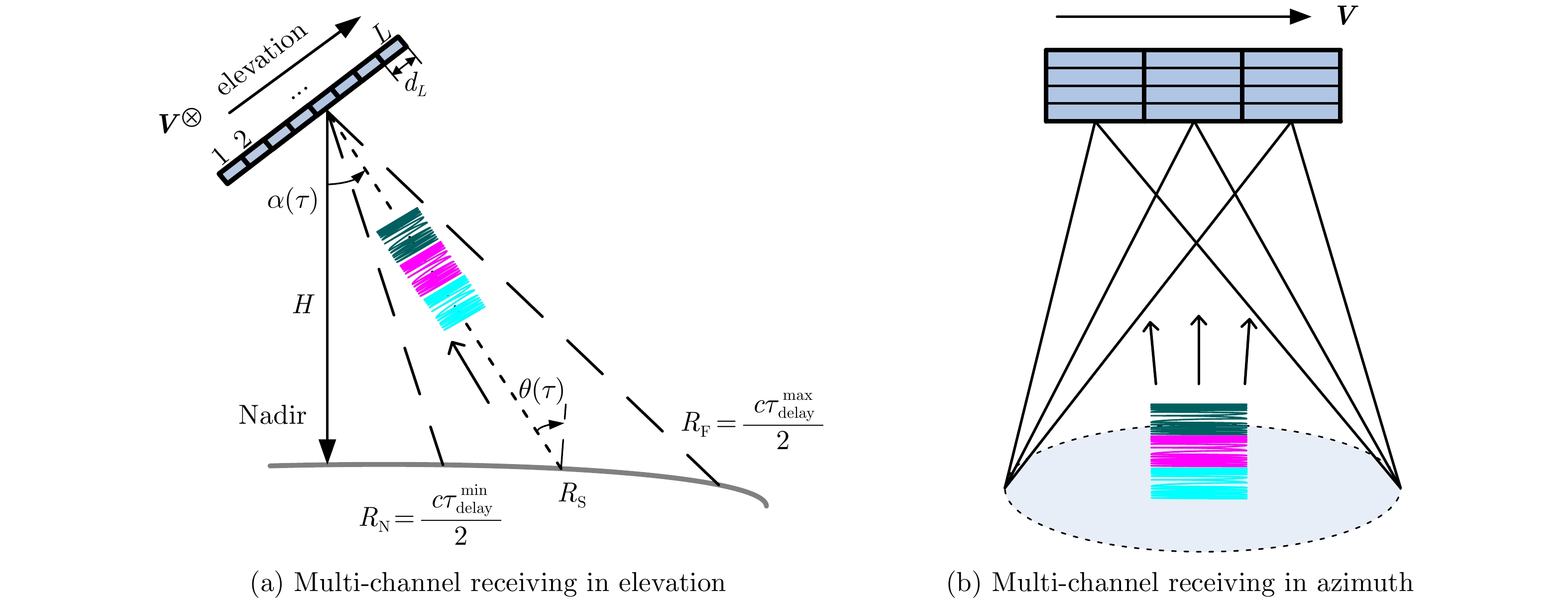
Figure 3. Cascaded DBF networks in elevation performing the SNR-preserving and interferences-free signal separation
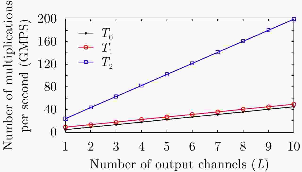
Figure 4. Number of real multiplications per second of the proposed two types of onboard DBF processing and the reference beamforming processing given in Ref. [8] (N=5 and P= 8)
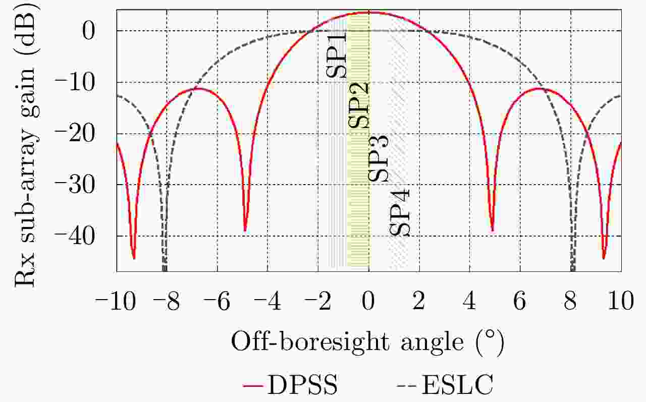
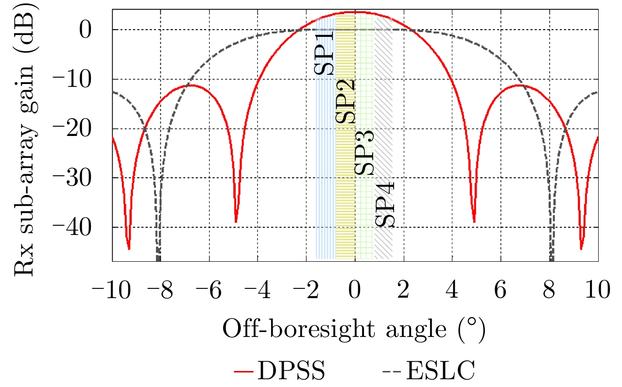
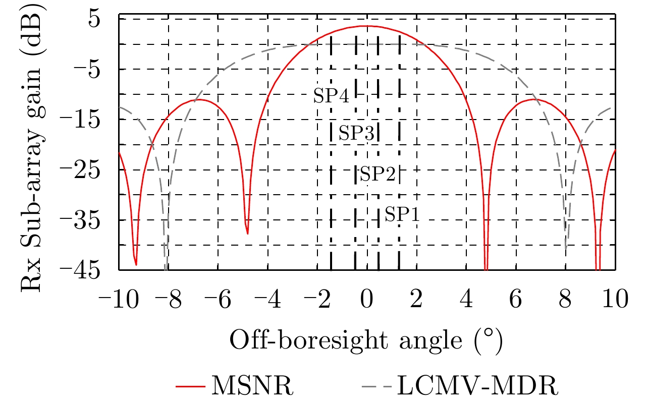
Figure 5. The array patterns of onboard Type-A beamforming at instantaneous time
$t = {\tau _{\rm{c}}}$ 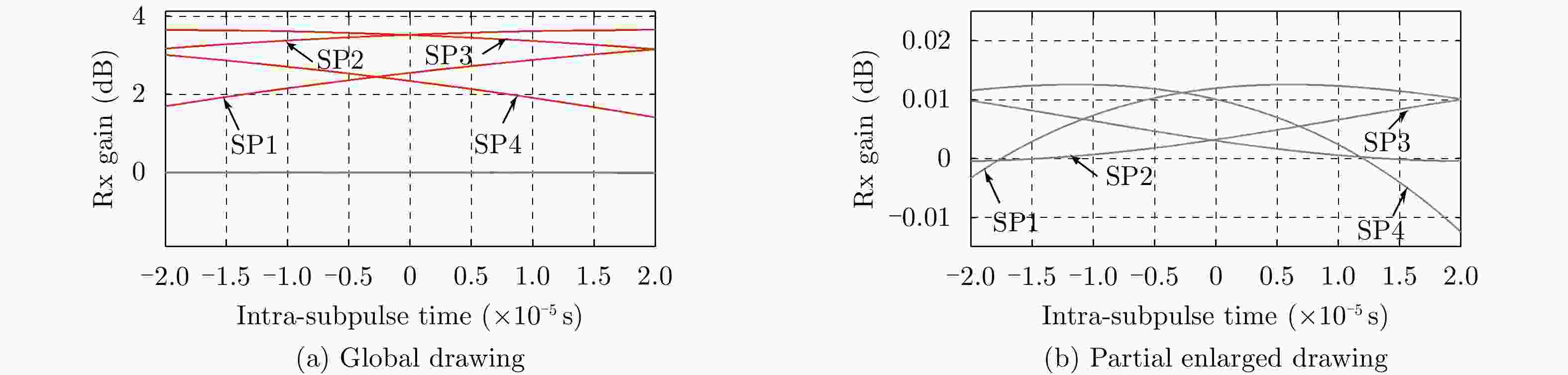
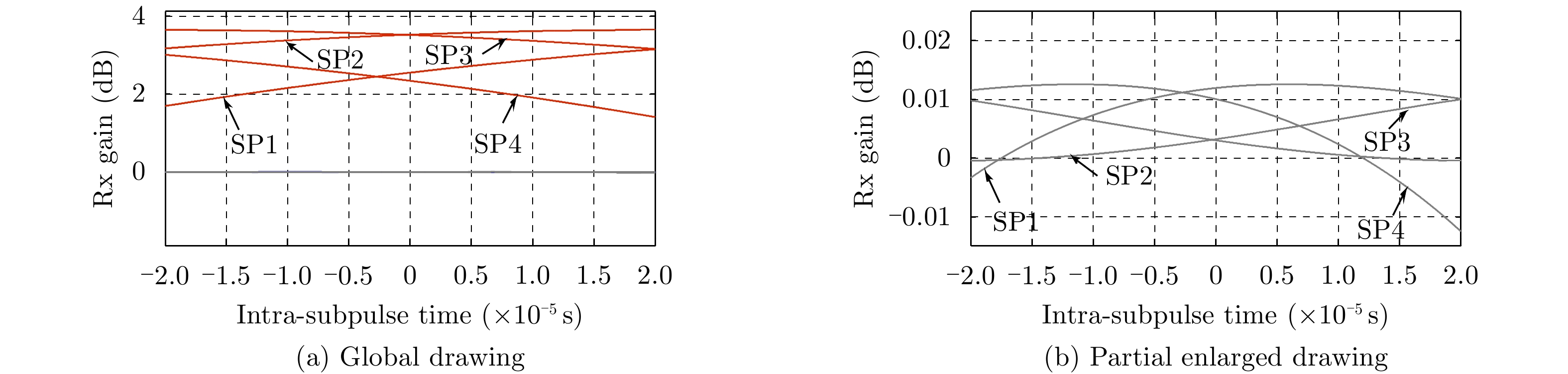
Figure 6. Amplitude of the distortion functions
$\mu _m^{(0)}(t)$ in the extent of each of 4 subpulses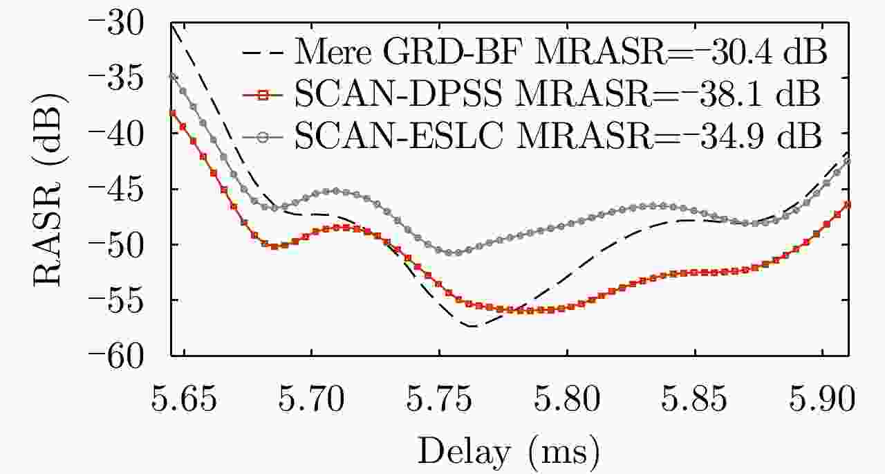
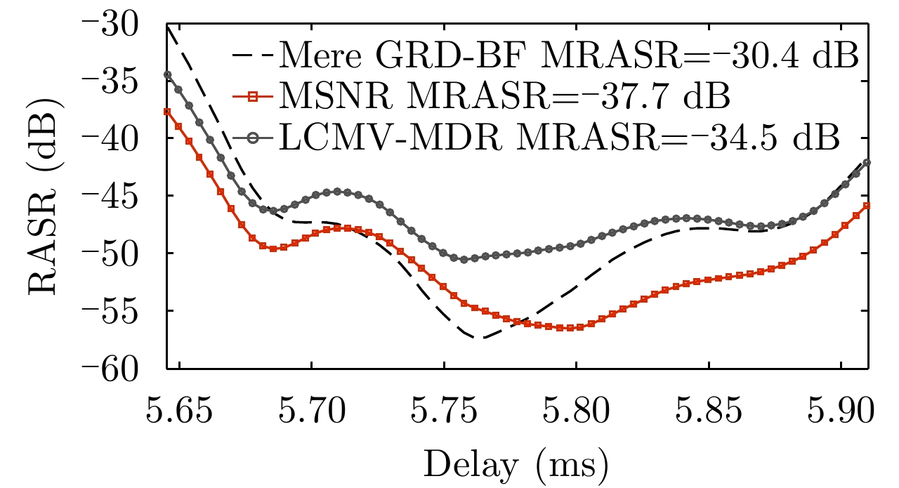
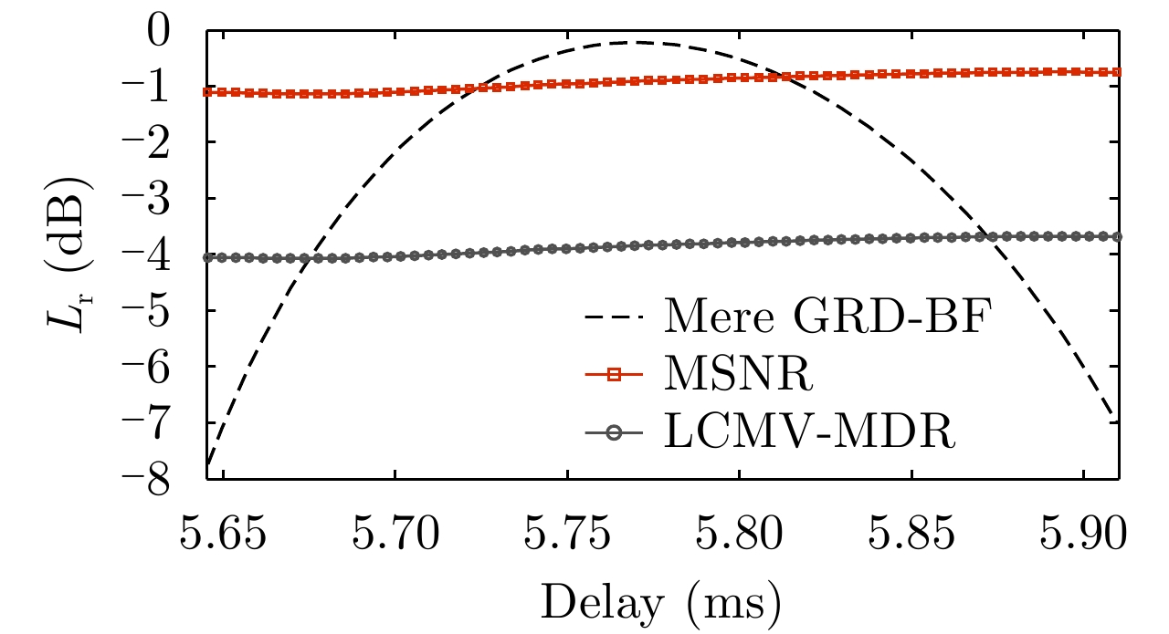
Figure 7. Performance comparison on RASR between the cascaded hybrid Type-A DBF networks and ground DBF in Ref. [8]
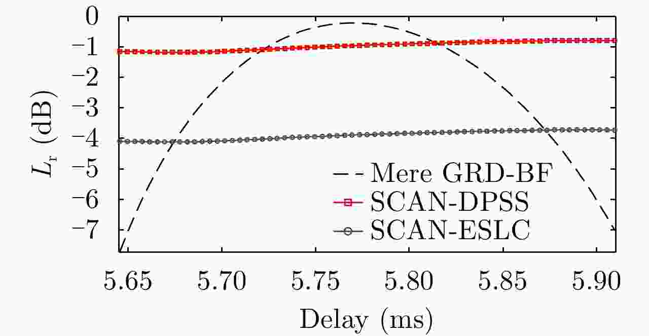
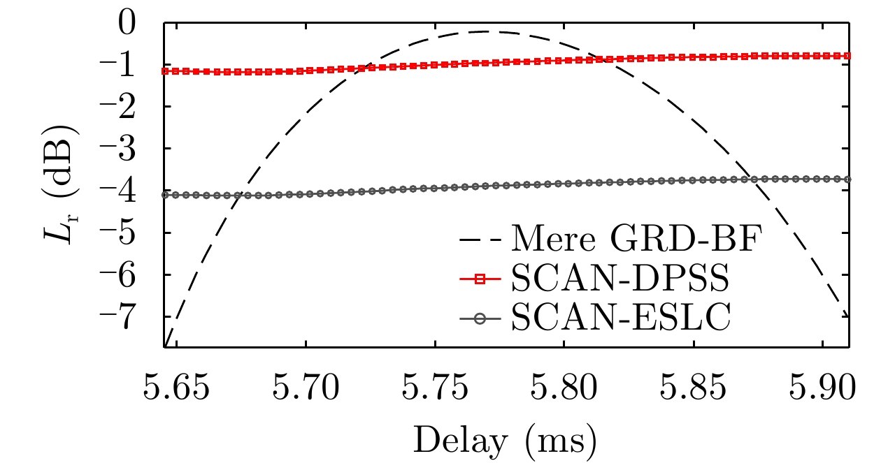
Figure 8. Performance comparison on SNR between the cascaded hybrid Type-A DBF networks and ground DBF in Ref. [8]
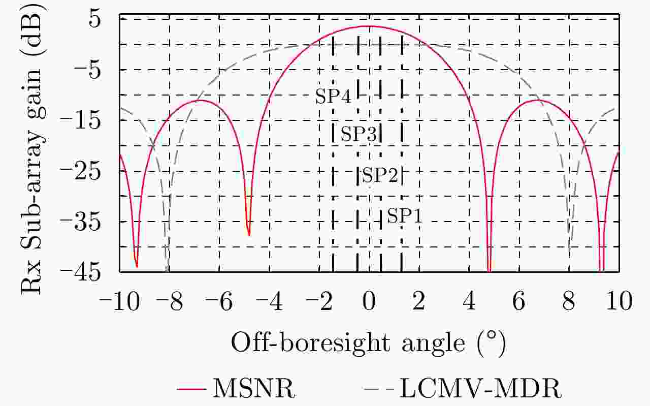
Figure 9. The array patterns of onboard Type-B beamforming at instantaneous time
$t = {\tau _{\rm{c}}}$ 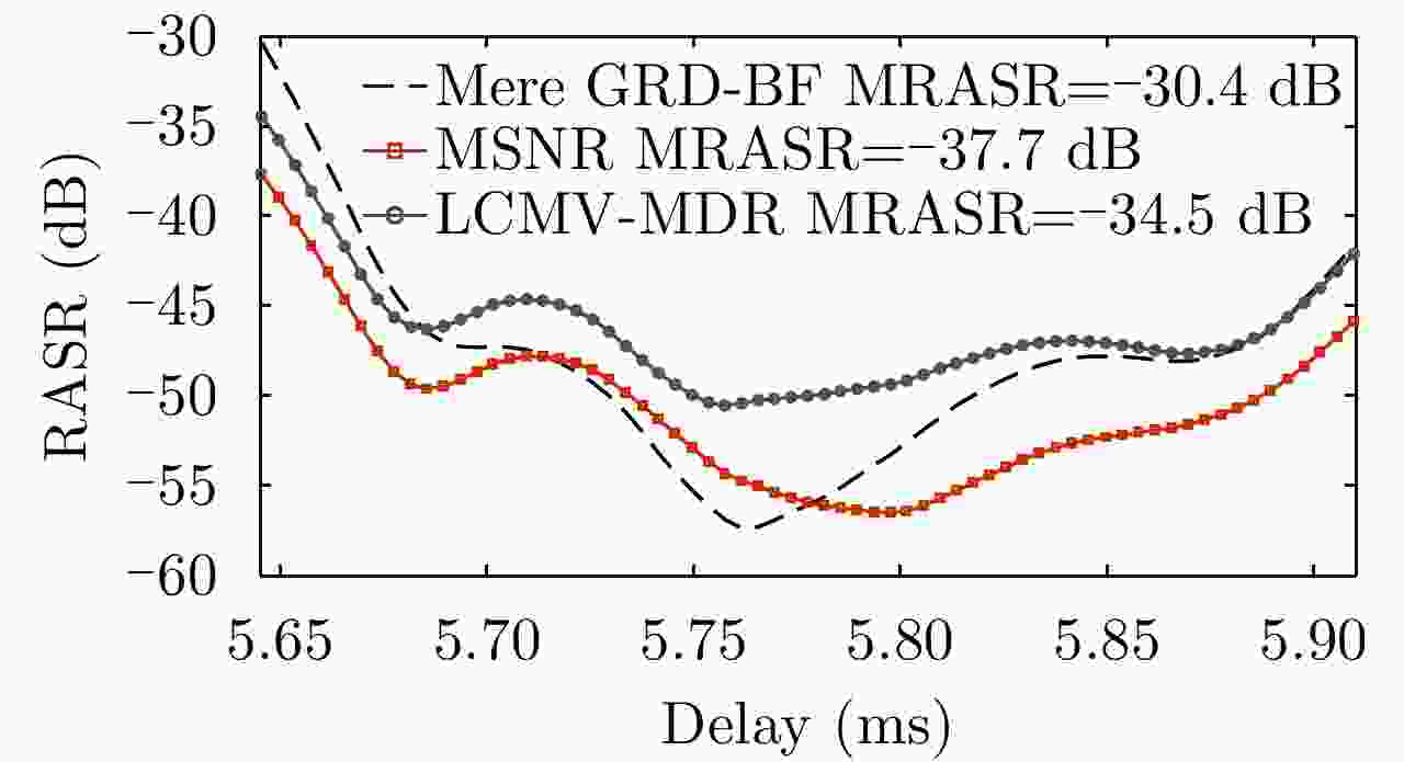
Figure 10. Performance comparison on RASR between the cascaded hybrid Type-B DBF networks and ground DBF in Ref. [8]
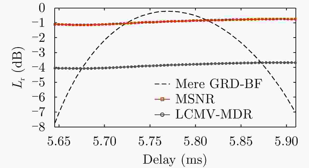
Figure 11. Performance comparison on SNR between the cascaded hybrid Type-B DBF networks and ground DBF in Ref. [8]
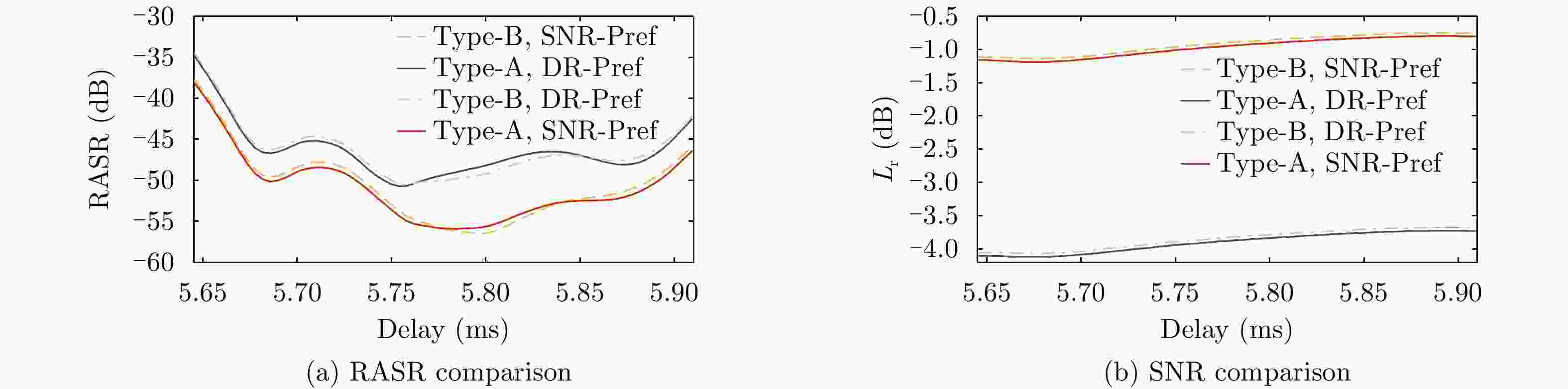
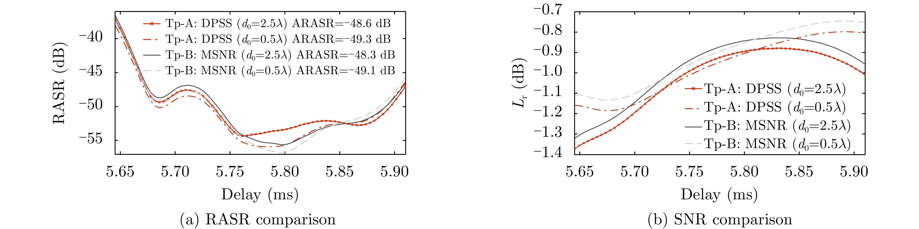
Figure 12. Across comparison of performance on RASR and SNR between the onboard transmit signal-structure-dependent beamformers (Type-B) and the non-signal-dependent ones (Type-A)

Figure 13. Performance on RASR and SNR for Type-A and Type-B SNR-preferred beamformers with an increased element spacing

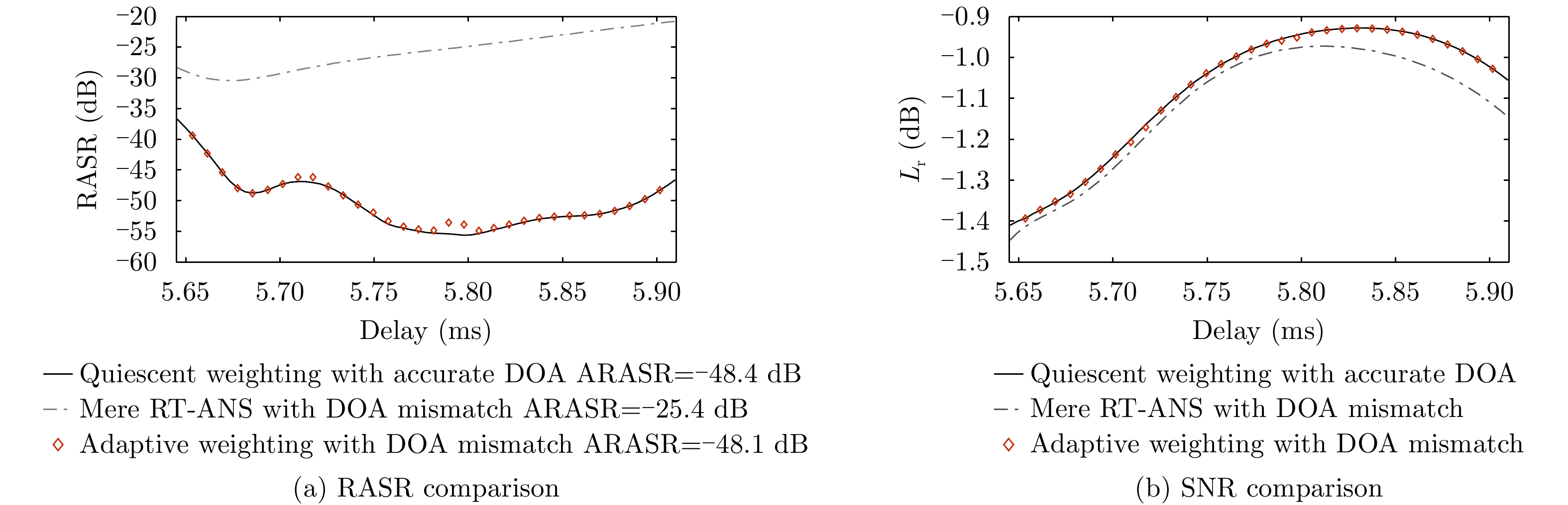
Figure 14. Performance on RASR and SNR of the cascaded DBF networks under the DOA mismatch condition in the presence of topographic height error, in comparison with the onboard real-time null-steering DBF in Ref. [7]
Table 1. Parameters used in the system simulation[8]
Parameter Value Parameter Value Wave length 0.031 m Number of subpulses 4 Swath width 100 km PRF 1310 Hz Off-nadir angle 18o~24o Azimuth subapertures 4 Azimuth resolution 1.5 m Antenna length 10.8 m Band width 250 MHz Antenna height 2.33 m Ground range resolution at center 1.5 m Processed Doppler bandwidth 4890 Hz Onboard elevation channel number 6 Azimuth ambiguity to signal ratio –30 dB Orbital altitude 800 km Subpulse duration/ interval 40 μs  下载: 导出CSV
-
[1] MOREIRA A, PRATS-IRAOLA P, YOUNIS M, et al. A tutorial on synthetic aperture radar[J]. IEEE Geoscience and Remote Sensing Magazine, 2013, 1(1): 6–43. doi: 10.1109/MGRS.2013.2248301 [2] KRIEGER G, GEBERT N, and MOREIRA A. Unambiguous SAR signal reconstruction from nonuniform displaced phase center sampling[J]. IEEE Geoscience and Remote Sensing Letters, 2004, 1(4): 260–264. doi: 10.1109/LGRS.2004.832700 [3] GEBERT N, KRIEGER G, and MOREIRA A. Digital beamforming on receive: Techniques and optimization strategies for high-resolution wide-swath SAR imaging[J]. IEEE Transactions on Aerospace and Electronic Systems, 2009, 45(2): 564–592. doi: 10.1109/TAES.2009.5089542 [4] KRIEGER G, GEBERT N, and MOREIRA A. Multidimensional waveform encoding: A new digital beamforming technique for synthetic aperture radar remote sensing[J]. IEEE Transactions on Geoscience and Remote Sensing, 2008, 46(1): 31–46. doi: 10.1109/TGRS.2007.905974 [5] ZHAO Qingchao, ZHANG Yi, WANG Wei, et al. Echo separation for space-time waveform-encoding SAR with digital scalloped beamforming and adaptive multiple null-steering[J]. IEEE Geoscience and Remote Sensing Letters, 2020, in press. doi: 10.1109/LGRS.2020.2968811 [6] FENG Fan, LI Shiqiang, YU Weidong, et al. Study on the processing scheme for space-time waveform encoding SAR system based on two-dimensional digital beamforming[J]. IEEE Transactions on Geoscience and Remote Sensing, 2012, 50(3): 910–932. doi: 10.1109/TGRS.2011.2162097 [7] FENG Fan, LI Shiqiang, YU Weidong, et al. Echo separation in multidimensional waveform encoding SAR remote sensing using an advanced null-steering beamformer[J]. IEEE Transactions on Geoscience and Remote Sensing, 2012, 50(10): 4157–4172. doi: 10.1109/TGRS.2012.2187905 [8] HE Feng, MA Xile, DONG Zhen, et al. Digital beamforming on receive in elevation for multidimensional waveform encoding SAR sensing[J]. IEEE Geoscience and Remote Sensing Letters, 2014, 11(12): 2173–2177. doi: 10.1109/LGRS.2014.2323267 [9] XU Wei and DENG Yunkai. Waveform diversity extraction in Spaceborne MIMO-SAR system based on multidimensional waveform encoding[J]. Journal of University of Electronic Science and Technology of China, 2012, 41(1): 25–30. doi: 10.3969/j.issn.1001-0548.2012.01.005 [10] HE Feng, DONG Zhen, and LIANG Diannong. A novel space-time coding Alamouti waveform scheme for MIMO-SAR[J]. IEEE Geoscience and Remote Sensing Letters, 2015, 12(2): 229–233. doi: 10.1109/LGRS.2014.2333232 [11] KRIEGER G. MIMO-SAR: Opportunities and pitfalls[J]. IEEE Transactions on Geoscience and Remote Sensing, 2014, 52(5): 2628–2645. doi: 10.1109/TGRS.2013.2263934 [12] YOUNIS M, KRIEGER G, and MOREIRA A. MIMO SAR techniques and trades[C]. 2013 IEEE European Radar Conference, Nuremberg, Germany, 2013: 141–144. [13] DIEBOLD A V, IMANI M F, and SMITH D R. Phaseless radar coincidence imaging with a MIMO SAR platform[J]. Remote Sensing, 2019, 11(5): 533. doi: 10.3390/rs11050533 [14] HUANG Pingping and XU Wei. ASTC-MIMO-TOPS mode with digital beam-forming in elevation for high-resolution wide-swath imaging[J]. Remote Sensing, 2015, 7(3): 2952–2970. doi: 10.3390/rs70302952 [15] KIM J, YOUNIS M, MOREIRA A, et al. Spaceborne MIMO synthetic aperture radar for multimodal operation[J]. IEEE Transactions on Geoscience and Remote Sensing, 2015, 53(5): 2453–2466. doi: 10.1109/TGRS.2014.2360148 [16] WANG Wenqin. MIMO SAR imaging: Potential and challenges[J]. IEEE Aerospace and Electronic Systems Magazine, 2013, 28(8): 18–23. doi: 10.1109/MAES.2013.6575407 [17] WANG Jie, LIANG Xingdong, DING Chibiao, et al. A novel scheme for ambiguous energy suppression in MIMO-SAR systems[J]. IEEE Geoscience and Remote Sensing Letters, 2015, 12(2): 344–348. doi: 10.1109/LGRS.2014.2340898 [18] QI Weikong and YU Weidong. A novel operation mode for spaceborne polarimetric SAR[J]. Science China Information Sciences, 2011, 54(4): 884–897. doi: 10.1007/s11432-011-4183-1 [19] YOUNIS M, HUBER S, PATYUCHENKO A, et al. Performance comparison of reflector- and planar-antenna based digital beam-forming SAR[J]. International Journal of Antennas and Propagation, 2009, 2009: 614931. [20] ZHAO Qingchao, ZHANG Yi, WANG Wei, et al. On the frequency dispersion in DBF SAR and digital scalloped beamforming[J]. IEEE Transactions on Geoscience and Remote Sensing, 2020, 58(5): 3619–3632. doi: 10.1109/TGRS.2019.2958863 [21] YOUNIS M, ROMMEL T, BORDONI F, et al. On the pulse extension loss in digital beamforming SAR[J]. IEEE Geoscience and Remote Sensing Letters, 2015, 12(7): 1436–1440. doi: 10.1109/LGRS.2015.2406815 [22] SUESS M and WIESBECK W. Side-looking synthetic aperture radar system[J]. European Patent EP, 2002, 1(241): 487. [23] BORDONI F, YOUNIS M, VARONA E M, et al. Performance investigation on scan-on-receive and adaptive digital beam-forming for high-resolution wide-swath synthetic aperture radar[C]. International ITG Workshop of Smart Antennas, Berlin, Germany, 2009: 114–121. [24] WANG Wei, WANG R, DENG Yunkai, et al. An improved processing scheme of digital beam-forming in elevation for reducing resource occupation[J]. IEEE Geoscience and Remote Sensing Letters, 2016, 13(3): 309–313. [25] OPPENHEIM A V, SCHAFER R W, and BUCK J R. Discrete-Time Signal Processing[M]. 2nd ed. Upper Saddle River: Prentice-Hall, 1999. [26] VAN TREES H L. Optimum Array Processing: Part IV of Detection, Estimation, and Modulation Theory[M]. New York, USA: Wiley-Interscience Press, 2002. [27] GUERCI J R. Theory and application of covariance matrix tapers for robust adaptive beamforming[J]. IEEE Transactions on Signal Processing, 1999, 47(4): 977–985. doi: 10.1109/78.752596 [28] GOLUB G H and VAN LOAN C F. Matrix Computations[M]. 2nd ed. Baltimore: The Johns Hopkins University Press, 1989. -


计量
- 文章访问数:
- HTML全文浏览量:
- PDF下载量:
- 被引次数: 0

