基于高斯混合聚类的阵列干涉SAR三维成像

李杭; 梁兴东; 张福博; 吴一戎

doi:10.12000/JR17020

基于高斯混合聚类的阵列干涉SAR三维成像

DOI: 10.12000/JR17020

李杭^1,2,3,,
梁兴东^1,2, ,,
张福博^1,2,,
吴一戎^1,2,

1.
微波成像技术重点实验室北京 100190
2.
中国科学院电子学研究所北京 100190
3.
中国科学院大学北京 100049

基金项目: 国家部委基金

详细信息

作者简介:
李杭：李杭(1989–)，男，江苏人，学士，中国科学技术大学；博士生，中国科学院电子学研究所；研究方向为阵列干涉SAR高精度3维成像。E-mail: aaronli@mail.ustc.edu.cn

梁兴东(1973–)，男，陕西人，博士，北京理工大学；研究员，中国科学院电子学研究所；研究方向为高分辨率合成孔径雷达系统、干涉合成孔径雷达、成像处理及应用、实时数字信号处理。E-mail: xdliang@mail.ie.ac.cn

张福博(1988–)，男，河北人，博士，中国科学院电子学研究所；助理研究员，研究方向为多通道SAR 3维重建、新体制雷达、阵列雷达信号处理。E-mail: zhangfubo8866@126.com

吴一戎(1963–)，男，安徽人，博士，中国科学院电子学研究所；研究员，中国科学院院士，中国科学院电子学研究所；研究方向为微波成像理论、微波成像技术和雷达信号处理。E-mail: wyr@mail.ie.ac.cn

通讯作者:
梁兴东 xdliang@mail.ie.ac.cn

中图分类号: TN957.52
计量
- 文章访问数: 3069
- HTML全文浏览量: 680
- PDF下载量: 576
- 被引次数: 8
出版历程
- 收稿日期: 2017-03-03
- 修回日期: 2017-04-10
- 网络出版日期: 2017-12-01

3D Imaging for Array InSAR Based on Gaussian Mixture Model Clustering

Li Hang^{1,2,3
,},
Liang Xingdong^{1,2
, ,},
Zhang Fubo^{1,2
,},
Wu Yirong^{1,2
,}

1.
Science and Technology on Microwave Imaging Laboratory, Beijing 100190, China
2.
Institute of Electronics, Chinese Academy of Sciences, Beijing 100190, China
3.
University of Chinese Academy of Sciences, Beijing 100049, China

Funds: The National Ministries Foundation

摘要

摘要:
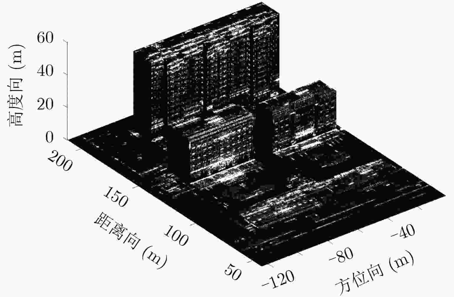
阵列干涉SAR具备高程分辨能力，单次航过即可生成观测场景的3维点云分布，解决叠掩问题。但是，由于阵列干涉SAR阵元数目有限、基线长度较短，高程向分辨率受到限制，加之城区建筑物的叠掩现象，常规方法重建结果定位精度较差，难以提取建筑物有效特征。针对这个问题，该文提出了一种基于高斯混合聚类的阵列干涉SAR 3维成像方法，首先通过基于压缩感知(Compressive Sensing, CS)的超分辨算法获得场景区域的3维点云分布，然后利用密度估计方法提取出建筑物的散射点，之后使用高斯混合模型(Gaussian Mixture Model, GMM)对建筑物3维点云进行聚类，最后利用系统参数完成各个区域的SAR图像反演，实现建筑物的3维成像。通过国内首次机载阵列干涉SAR实验的实际数据，验证了该文算法的有效性，并获得了真实的建筑物3维成像结果。
- 3维成像 /
- 阵列干涉SAR /
- 叠掩现象 /
- 压缩感知 /
- 高斯混合模型聚类
Abstract:
Array InSAR can generate 3D point clouds with the use of SAR images of the observed scene, which are obtained using multiple channels in a single flight. Its resolution power in elevation enables one to solve the layover problem. However, due to the limited number of arrays and the short baseline length, the resolution power in elevation is restricted. Together with the layover phenomenon of the urban buildings, the result of 3D reconstruction suffers from poor accuracy in positioning, and it is difficult to extract the effective characteristics of the buildings. In view of this situation, this paper proposed a 3D reconstruction method of array InSAR based on Gaussian mixture model clustering. First, the 3D point clouds of the observed scene are obtained by an algorithm with super-resolution based on compressive sensing, and then the scatters of buildings are extracted by density estimation; after which the method of Gaussian mixture model clustering is used to classify the 3D point clouds of the buildings. Finally, the inverse SAR images of each region are obtained by using the system parameters, and the 3D reconstruction of the buildings is completed. Based on the actual data of the first domestic 3D imaging experiment by airborne array InSAR, the validity of the algorithm is confirmed and the 3D imaging results of the buildings are obtained.
- 3D reconstruction /
- Array InSAR /
- Layover phenomenon /
- Compressive Sensing (CS) /
- Gaussian Mixture Model clustering (GMM clustering)

HTML全文

1. Introduction

In recent years, Frequency Diverse Array (FDA) radar has received much attention due to its range-angle-time-dependent beampattern^[1,2]. Combining the advantages of FDA and traditional phased array Multiple-Input Multiple-Output (MIMO) radar in the degree of freedom, the FDA Multiple-Input Multiple Output (FDA-MIMO) radar was proposed in Ref. [3] and applied in many fields^[4-9]. For parameter estimation algorithm, the authors first proposed a FDA-MIMO target localization algorithm based on sparse reconstruction theory^[10], and an unbiased joint range and angle estimation method was proposed in Ref. [11]. The work of Ref. [12] further proved that the FDA-MIMO is superior to traditional MIMO radar in range and angle estimation performance, and the authors of Ref. [13] introduced a super-resolution MUSIC algorithm for target location, and analyzed its resolution threshold. Meanwhile, high-resolution Doppler processing is utilized for moving target parameter estimation^[14]. The Estimation of Signal Parameters via Rotational Invariance Technique (ESPRIT) and PARAllel FACtor (PARAFAC) was proposed in Ref. [15], which is a search-free algorithm for FDA-MIMO.

Moreover, the research of conformal array has received more and more attention. Conformal array is a non-planar array that can be completely attached to the surface of the carrier^[16]. It has significant advantages such as reducing the aerodynamic impact on the carrier and smaller radar cross section^[17]. In addition, conformal array can achieve wide-angle scanning with a lower SideLobe Level (SLL)^[18]. Different from traditional arrays, the element beampattern of conformal array needs to be modeled separately in the parameter estimation due to the difference of carrier curvature^[19-21].

As far as we know, most of the existing researches on FDA-MIMO are based on linear array, while there is little research on the combination of FDA-MIMO and conformal array^[22]. In this paper, we replace the receiving array in the traditional FDA-MIMO with conformal array. Compared with conventional FDA-MIMO, conformal FDA-MIMO inherits the merits of conformal array and FDA-MIMO, which can effectively improve the stealth and anti-stealth performance of the carrier, and reduce the volume and the air resistance of the carrier. For conformal FDA-MIMO, we further study the parameters estimation algorithm. The major contributions of this paper are summarized as follows:

(1) A conformal FDA-MIMO radar model is first formulated.

(2) The parameter estimation Cramér-Rao Lower Bound (CRLB) for conformal FDA-MIMO radar is derived.

(3) Inspired by the existing work of Refs. [23,24], a Reduced-Dimension MUSIC (RD-MUSIC) algorithm for conformal FDA-MIMO radar is correspondingly proposed to reduce the complexity.

The rest of the paper consists of four parts. Section 2 formulates the conformal FDA-MIMO radar model, and Section 3 derives a RD-MUSIC algorithm for conformal FDA-MIMO radar. Simulation results for conformal FDA-MIMO radar with semi conical conformal receiving array are provided in Section 4. Finally, conclusions are drawn in Section 5.

2. Conformal FDA-MIMO Radar

2.1 General conformal FDA-MIMO signal model

For the convenience of analysis, we consider a monostatic conformal FDA-MIMO radar which is composed by a $M$ -element linear FDA transmitting array and a $N$ -element conformal receiving array, as shown in Fig. 1. d denotes the inter-element spacing, the carrier frequency at the mth transmitting element is ${f_m} = {f_1} + \Delta f(m - 1)$ , $m = 1,2, \cdots ,M$ where ${f_1}$ is the transmission frequency of the first antenna element, which is called as reference frequency, and $\Delta f$ is the frequency offset between the adjacent array elements.

Figure 1. Conformal FDA-MIMO radar

DownLoad: Full-Size Img PowerPoint

The complex envelope of the transmitted signal of the mth transmitting element is denoted as ${{\varphi _m}} (t)$ , assume the transmitting waveforms have orthogonality,

$\int_{{T_p}} {{\varphi _m}} (t)\varphi _{{m_1}}^*(t - \tau ){\rm{d}}t = 0,\quad {m_1} \ne m$

(1)

where $\tau$ denotes the time delay, ${T_p}$ denotes the pulse duration, and ${\left( \cdot \right)^ * }$ is conjugate operator. The signal transmitted from the mth element can be expressed as

${s_m}(t) = {a_m}(t,\theta ,\phi ,r){\varphi _m}(t),\quad 0 \le t \le {T_p}$

(2)

where

$\begin{split} & {a_m}(t,\theta ,\phi ,r) \hfill \\ & =\exp \left\{ { - {\rm{j}}2\pi \left( \begin{gathered} \frac{{(m - 1)\Delta fr}}{{\rm{c}}} - \frac{{{f_1}(m - 1){{d}}\sin \alpha }}{{\rm{c}}} \hfill \\ - (m - 1)\Delta ft \hfill \\ \end{gathered} \right)} \right\} \end{split}$

(3)

is the mth element of the transmitting steering vector according to the phase difference between adjacent elements, the angle between far-field target and transmitting array is denoted as $\alpha = \arcsin (\sin \theta \cos \phi )$ , where $\arcsin ( \cdot )$ denotes arcsine operator, $\alpha$ can be calculated by using the inner product between the target vector and unit vector along the $X$ -axis. $\theta ,\phi ,r$ are the elevation, azimuth and range between the target and the origin point, respectively. The phase difference between adjacent elements is

$\Delta {\psi _{t0}} = 2\pi \left( {\frac{{\Delta fr}}{{\rm{c}}} - \frac{{{f_1}d\sin \alpha }}{{\rm{c}}} - \Delta ft} \right)$

(4)

where ${\rm{c}}$ is light speed. For far-field target ${P}\left( {r,\theta ,\phi } \right)$ , the transmitting steering vector is

$\begin{split} {{\boldsymbol{a}}_0}\left( {t,\theta ,\phi ,r} \right) =& \left[ {1,\exp \left\{ { - {\rm{j}}\Delta {\psi _{t0}}} \right\}, \cdots ,} \right. \\ &{\left. {\exp \left\{ { - {\rm{j}}(M - 1)\Delta {\psi _{t0}}} \right\}} \right]^{\rm{T}}} \end{split}$

(5)

For the conformal receiving array, as shown in Fig. 1(b), the time delay between target ${P}\left( {r,\theta ,\phi } \right)$ and the nth receiving array element is

${\tau _n} = {r_n}/{\rm{c}}$

(6)

where ${r_n}$ is the range between target and the nth receiving array element. For far-field assumption, the ${r_n}$ can be approximated as

${r_n} \approx r - {\vec {\boldsymbol{p}}_n} \cdot \vec {\boldsymbol{r}}$

(7)

where r denotes the range between the target and the origin point, ${\vec {\boldsymbol{p}}_n} = {x_n}{{\boldsymbol{e}}_x} + {y_n}{{\boldsymbol{e}}_y} + {z_n}{{\boldsymbol{e}}_z}$ denotes the position vector from the nth element to origin point, and $\vec {\boldsymbol{r}} = \sin \theta \cos \phi {{\boldsymbol{e}}_x} + \sin \theta \sin \phi {{\boldsymbol{e}}_y} + \cos\theta {{\boldsymbol{e}}_z}$ is the unit vector in target orientation, where ${{\boldsymbol{e}}_x},{{\boldsymbol{e}}_y}$ and ${{\boldsymbol{e}}_z}$ are the unit vectors along the X- , Y- , and $Z$ -axis, respectively. $({x_n},{y_n},{z_n})$ are the coordinates of the nth element in the Cartesian coordinate system. For simplicity, we let $u = \sin \theta \cos \phi$ , $v = \sin \theta \cos \phi$ , so the time delay ${\tau _n} =$ $(r - (u{x_n} + v{y_n} + \cos \theta {z_n}))/{\rm{c}}$ . The time delay between the first element and the nth element at the receiving array is expressed as

$\begin{split} \Delta {\tau _{{r_n}}} =& {\tau _1} - {\tau _n} \\ =& \frac{{u({x_n} - {x_1}) + v({y_n} - {y_1}) + \cos \theta ({z_n} - {z_1})}}{{\rm{c}}} \\ \end{split}$

(8)

And the corresponding phase difference between the first element and the nth element is

$\Delta {\psi _{{R_n}}} = 2\pi {f_1}\Delta {\tau _{{r_n}}}$

(9)

Consequently, the receiving steering vector is

$\begin{split} {\boldsymbol{b}}\left( {\theta ,\phi } \right) =& \left[ {{r_1}(\theta ,\phi ),{r_2}(\theta ,\phi )\exp (j\Delta {\psi _{{r_2}}}), \cdots ,} \right. \\ &{\left. {{r_N}(\theta ,\phi )\exp({\rm{j}}\Delta {\psi _{{r_N}}})} \right]^{\rm{T}}} \\ \end{split}$

(10)

where ${r_n}(\theta ,\phi )$ is the nth conformal receiving array element beampattern which should be designed in its own local Cartesian coordinate system. In this paper, we utilize Euler rotation method to establish transformation frame between local coordinate system and global coordinate system^[25,26].

Then the total phase difference between adjacent transmitting array elements can be rewritten as

$\Delta {\psi _t} = 2\pi \left( {\frac{{\Delta f2r}}{{\rm{c}}} - \frac{{{f_1}d\sin \alpha }}{{\rm{c}}} - \Delta ft} \right)$

(11)

where the factor $2r$ in the first term represents the two-way transmission and reception, and the correspondingly transmitting steering vector is written as

$\begin{split} {\boldsymbol{a}}\left( {t,\theta ,\phi ,r} \right) =& \left[ {1,\exp \left\{ { - {\rm{j}}\Delta {\psi _t}} \right\}, \cdots ,} \right. \\ & {\left. {\exp \left\{ { - {\rm{j}}(M - 1)\Delta {\psi _t}} \right\}} \right]^{\rm{T}}} \end{split}$

(12)

Assuming L far-field targets are located at $\left( {{\theta _i},{\phi _i},{R_i}} \right)$ , $i = 1,2,\cdots,L$ and snapshot number is $K$ . After matched filtering, the received signal can be formulated as following matrix (13,14)

${\boldsymbol{X = AS + N}}$

(13)

where the array manifold ${\boldsymbol{A}}$ is expressed as

$\begin{split} {\boldsymbol{A}} = &\left[ {{{\boldsymbol{a}}_{t,r}}\left( {{\theta _1},{\phi _1},{r_1}} \right), \cdots ,{{\boldsymbol{a}}_{t,r}}\left( {{\theta _L},{\phi _L},{r_L}} \right)} \right] \hfill \\ =& \left[ {\boldsymbol{b}}\left( {{\theta _1},{\phi _1}} \right) \otimes {\boldsymbol{a}}\left( {{\theta _1},{\phi _1},{r_1}} \right), \cdots ,{\boldsymbol{b}}\left( {{\theta _L},{\phi _L}} \right) \right.\\ & \left.\otimes {\boldsymbol{a}}\left( {{\theta _L},{\phi _L},{r_L}} \right) \right] \end{split}$

(14)

where ${{\boldsymbol{a}}_{t,r}}\left( {\theta ,\phi ,r} \right)$ is the joint transmitting-receiving steering vector, ${\boldsymbol{S}} = \left[ {s({t_1}),s({t_2}), \cdots ,s({t_K})} \right] \in {\mathbb{C}^{L \times K}}$ and ${\boldsymbol{N}} \in {\mathbb{C}^{MN \times K}}$ denote the signal matrix and noise matrix, respectively, where noise follows the independent identical distribution, and $\otimes$ denotes Kronecker product.

$\begin{split} {\boldsymbol{a}}\left( {\theta ,\phi ,r} \right) =& \left[ 1\; {\exp \left\{ { - {\rm{j}}2\pi \left( {\dfrac{{2\Delta fr}}{{\rm{c}}} - \dfrac{{{f_1}d\sin \alpha }}{{\rm{c}}}} \right)} \right\}} \right. \hfill \\ &\left. \cdots {\exp \left\{ { - {\rm{j}}2\pi (M - 1)\left( {\dfrac{{2\Delta fr}}{{\rm{c}}} - \dfrac{{{f_1}d\sin \alpha }}{{\rm{c}}}} \right)} \right\}} \right] \end{split}$

(15)

which can be expressed as

${\boldsymbol{a}}\left( {\theta ,\phi ,r} \right) = {\boldsymbol{a}}\left( {\theta ,\phi } \right) \odot {\boldsymbol{a}}\left( r \right)$

(16)

where

$\begin{split} {\boldsymbol{a}}(r) =& \left[ {1,\exp \left( - {\rm{j}}2\pi \frac{{2\Delta fr}}{{\rm{c}}}\right), \cdots ,} \right. \\ & {\left. {\exp\left( { - {\rm{j}}2\pi (M - 1)\frac{{2\Delta fr}}{{\rm{c}}}} \right)} \right]^{\rm{T}}}\qquad \end{split}$

(17)

$\begin{split} {\boldsymbol{a}}(\theta ,\phi ) =& \left[ {1,\exp \left({\rm{j}}2\pi \frac{{{f_1}d\sin \alpha }}{{\rm{c}}}\right),} \cdots ,\right. \hfill \\ &{\left. { \exp \left[{\rm{j}}2\pi (M - 1)\frac{{{f_1}d\sin \alpha }}{{\rm{c}}}\right]} \right]^{\rm{T}}} \end{split}$

(18)

and $\odot$ represents Hadamard product operator.

2.2 CRLB of conformal FDA-MIMO

The CRLB can be obtained from the inverse of Fisher information matrix^[27,28], which establishes a lower bound for the variance of any unbiased estimator. We employ the CRLB for conformal FDA-MIMO parameter estimation to evaluate the performance of some parameter estimation algorithms.

The discrete signal model is

${\boldsymbol{x}}[k] = {{\boldsymbol{a}}_{t,r}}(\theta ,\phi ,r)s[k] + {\boldsymbol{N}}[k],\quad k = 1,2, \cdots ,K$

(19)

For the sake of simplification, we take ${{\boldsymbol{a}}_{t,r}}$ as the abbreviation of ${{\boldsymbol{a}}_{t,r}}(\theta ,\phi ,r)$ .

The Probability Distribution Function (PDF) of the signal model with $K$ snapshots is

$\begin{split} p({\boldsymbol{x}}\left| {\theta ,\phi ,r} \right.) =& \frac{1}{{{{(2\pi \sigma _n^2)}^{\textstyle\frac{K}{2}}}}} \\ & \cdot \exp \left( - \frac{1}{{\sigma _n^2}}{({\boldsymbol{x}} - {{\boldsymbol{a}}_{t,r}}{\boldsymbol{s}})^{\rm{H}}}({\boldsymbol{x}} - {{\boldsymbol{a}}_{t,r}}{\boldsymbol{s}})\right) \\ \end{split}$

(20)

where ${\boldsymbol{x}} = [{\boldsymbol{x}}(1),{\boldsymbol{x}}(2),\cdots,{\boldsymbol{x}}(K)]$ and ${\boldsymbol{s}} = [s(1),$ $s(2), \cdots,s(K)]$ .

The CRLB matrix form of elevation angle, azimuth angle and range is given by Eq. (21), diagonal elements $\left\{ {{C_{\theta \theta }},{C_{\phi\phi} } ,{C_{rr}}} \right\}$ represent CRLB of estimating elevation angle, azimuth angle and range, respectively.

$\begin{split} {\rm{CRLB}} = &\left[ {\begin{array}{*{20}{c}} {{C_{\theta \theta }}}&{{C_{\theta \phi }}}&{{C_{\theta r}}} \\ {{C_{\phi \theta }}}&{{C_{\phi\phi} } }&{{C_{\phi r}}} \\ {{C_{r\theta }}}&{{C_{r\phi }}}&{{C_{rr}}} \end{array}} \right] \\ =& {{\rm{FIM}}^{ - 1}} = \left[ {\begin{array}{*{20}{c}} {{F_{11}}}&{{F_{12}}}&{{F_{13}}} \\ {{F_{21}}}&{{F_{22}}}&{{F_{23}}} \\ {{F_{31}}}&{{F_{32}}}&{{F_{33}}} \end{array}} \right] \end{split}$

(21)

The elements of Fisher matrix can be expressed as

${F_{ij}} = - E\left[ {\dfrac{{{\partial ^2}\ln (p(x\mid \theta ,\phi ,r))}}{{\partial {x_i}\partial {x_j}}}} \right],\quad i,j = 1,2,3$

(22)

In the case of $K$ snapshots, PDF can be rewritten as

$\begin{split} p({\boldsymbol{x}}\left| {\theta ,\phi ,r} \right.) =& C\exp \left\{ { - \frac{1}{{\sigma _n^2}}} \right.\sum\limits_{n = 1}^K {{{\bigr({\boldsymbol{x}}[k] - {{\boldsymbol{a}}_{t,r}}s[k]\bigr)}^{\rm{H}}}} \\ & { \cdot \bigr({\boldsymbol{x}}[k] - {{\boldsymbol{a}}_{t,r}}s[k]\bigr)} \} \\[-18pt] \end{split}$

(23)

where $C$ is a constant, natural logarithm of Eq. (23) is

$\begin{split} \ln (p({\boldsymbol{x}}\left| {\theta ,\phi ,r} \right.)) =& \ln (C) - \frac{1}{{\sigma _n^2}}\sum\limits_{k = 1}^K {{{\bigr({\boldsymbol{x}}[k] - {{\boldsymbol{a}}_{t,r}}s[k]\bigr)}^{\rm{H}}}} \\ & \cdot \bigr({\boldsymbol{x}}[k] - {{\boldsymbol{a}}_{t,r}}s[k]\bigr) \\[-10pt] \end{split}$

(24)

where $\ln ( \cdot )$ represents the logarithm operator. The first entry of Fisher matrix can be expressed as

${F_{11}} = - E\left[ {\frac{{{\partial ^2}\ln (p({\boldsymbol{x}}\left| {\theta ,\phi ,r} \right.))}}{{\partial {\theta ^2}}}} \right]$

(25)

Correspondingly, the first derivative of natural logarithm is given by

$\begin{split} \frac{{\partial \ln (p({\boldsymbol{x}}\left| {\theta ,\phi ,r} \right.))}}{{\partial \theta }} =& - \frac{1}{{\sigma _n^2}}\sum\limits_{k = {\text{1}}}^K {\left( { - {{\boldsymbol{x}}^{\rm{H}}}\left[ k \right]\frac{{\partial {{\boldsymbol{a}}_{t,r}}}}{{\partial \theta }}s\left[ k \right]} \right.} \hfill \\ & - \frac{{\partial {\boldsymbol{a}}_{t,r}^{\rm{H}}}}{{\partial \theta }}s\left[ k \right]{\boldsymbol{x}}\left[ k \right] + \frac{{\partial {\boldsymbol{a}}_{t,r}^{\rm{H}}}}{{\partial \theta }}{{\boldsymbol{a}}_{t,r}}{s^2}\left[ n \right]{\boldsymbol{a}} \hfill \\ &\left. { + {\boldsymbol{a}}_{t,r}^{\rm{H}}\frac{{\partial {{\boldsymbol{a}}_{t,r}}}}{{\partial \theta }}{s^2}\left[ n \right]} \right) \\[-20pt] \end{split}$

(26)

Then we can obtain the second derivative of

$\begin{split} & \frac{{{\partial ^2}\ln (p({\boldsymbol{x}}\left| {\theta ,\phi ,r} \right.))}}{{\partial {\theta ^2}}} \hfill \\ & \quad= - \frac{1}{{\sigma _n^2}}\sum\limits_{k = {\text{1}}}^K {\left( { - {\boldsymbol{x}}{{\left[ k \right]}^{\rm{H}}}\frac{{{\partial ^2}{{\boldsymbol{a}}_{t,r}}}}{{\partial {\theta ^2}}}s\left[ k \right]} \right.} \hfill \\ & \qquad - \frac{{{\partial ^2}{\boldsymbol{a}}_{t,r}^{\rm{H}}}}{{\partial {\theta ^2}}}s\left( k \right){\boldsymbol{x}}\left[ k \right] \hfill + \frac{{{\partial ^2}{\boldsymbol{a}}_{t,r}^{\rm{H}}}}{{\partial {\theta ^2}}}{{\boldsymbol{a}}_{t,r}}s{\left[ k \right]^2} \\ & \qquad+ \frac{{\partial {\boldsymbol{a}}_{t,r}^{\rm{H}}}}{{\partial \theta }}\frac{{\partial {{\boldsymbol{a}}_{t,r}}}}{{\partial \theta }}s{\left[ k \right]^2} + \frac{{\partial {\boldsymbol{a}}_{t,r}^{\rm{H}}}}{{\partial \theta }}\frac{{\partial {{\boldsymbol{a}}_{t,r}}}}{{\partial \theta }}s{{\left[ k \right]}^2} \\ & \qquad \left.+ {\boldsymbol{a}}_{t,r}^{\rm{H}}\frac{{{\partial ^2}{{\boldsymbol{a}}_{t,r}}}}{{\partial {\theta ^2}}}s{{\left[ k \right]}^2} \right) \end{split}$

(27)

And then we have

$\begin{split} \sum\limits_{k = 1}^K {\boldsymbol{x}} [k] =& \sum\limits_{k = 1}^K {{{\boldsymbol{a}}_{t,r}}s[k] + {\boldsymbol{N}}[k]} \\ =& {{\boldsymbol{a}}_{t,r}}(\theta ,\phi ,r)\sum\limits_{k = 1}^K s [k] \end{split}$

(28)

and

$\sum\limits_{k = 1}^K {{s^2}} [k] = K{{\rm{var}}} (s[k]) = K\sigma _s^2$

(29)

where ${{\rm{var}}} ( \cdot )$ is a symbol of variance. Therefore, the PDF after quadratic derivation can be written as

$\begin{split} &E\left[ {\frac{{{\partial ^2}\ln (p({\boldsymbol{x}}\left| {\theta ,\phi ,r} \right.))}}{{\partial {\theta ^2}}}} \right] \hfill \\ & \quad=- \frac{{K\sigma _s^2}}{{\sigma _n^2}}\left( {\frac{{\partial {\boldsymbol{a}}_{t,r}^{\rm{H}}}}{{\partial \theta }}\frac{{\partial {{\boldsymbol{a}}_{t,r}}}}{{\partial \theta }} + \frac{{\partial {\boldsymbol{a}}_{t,r}^{\rm{H}}}}{{\partial \theta }}\frac{{\partial {{\boldsymbol{a}}_{t,r}}}}{{\partial \theta }}} \right) \\ & \quad= - \frac{{2K\sigma _s^2}}{{\sigma _n^2}}{\left\| {\frac{{\partial {{\boldsymbol{a}}_{t,r}}}}{{\partial \theta }}} \right\|^2} \end{split}$

(30)

where $\left\| \cdot \right\|$ denotes 2-norm. Similarly, the other elements of the Fisher matrix can also be derived in the similar way, so the Fisher matrix can be expressed as

$\begin{split} {{\rm{CRLB}}^{ - 1}} = & {\rm{FIM}} = \frac{{2K\sigma _s^2}}{{\sigma _n^2}} \\ & \cdot \left[ {\begin{array}{*{20}{c}} {{{\left\| {\dfrac{{\partial {\boldsymbol{a}}}}{{\partial \theta }}} \right\|}^2}}&{{{\rm{FIM}}_{12}}}&{{{\rm{FIM}}_{13}}} \\ {{{\rm{FIM}}_{21}}}&{{{\left\| {\dfrac{{\partial {\boldsymbol{a}}}}{{\partial \phi }}} \right\|}^2}}&{{{\rm{FIM}}_{23}}} \\ {{{\rm{FIM}}_{31}}}&{{{\rm{FIM}}_{32}}}&{{{\left\| {\dfrac{{\partial {\boldsymbol{a}}}}{{\partial r}}} \right\|}^2}} \end{array}} \right] \end{split}$

(31)

where

${{\rm{FIM}}_{12}} = \frac{1}{2}\left[ {\frac{{\partial {\boldsymbol{a}}_{t,r}^{\rm{H}}}}{{\partial \theta }}\frac{{\partial {{\boldsymbol{a}}_{t,r}}}}{{\partial \phi }} + \frac{{\partial {\boldsymbol{a}}_{t,r}^{\rm{H}}}}{{\partial \phi }}\frac{{\partial {{\boldsymbol{a}}_{t,r}}}}{{\partial \theta }}} \right],$

${{\rm{FIM}}_{13}} = \frac{1}{2}\left[ {\frac{{\partial {\boldsymbol{a}}_{t,r}^{\rm{H}}}}{{\partial \theta }}\frac{{\partial {{\boldsymbol{a}}_{t,r}}}}{{\partial r}} + \frac{{\partial {\boldsymbol{a}}_{t,r}^{\rm{H}}}}{{\partial r}}\frac{{\partial {{\boldsymbol{a}}_{t,r}}}}{{\partial \theta }}} \right],$

${{\rm{FIM}}_{21}} = \frac{1}{2}\left[ {\frac{{\partial {\boldsymbol{a}}_{t,r}^{\rm{H}}}}{{\partial \phi }}\frac{{\partial {{\boldsymbol{a}}_{t,r}}}}{{\partial \theta }} + \frac{{\partial {\boldsymbol{a}}_{t,r}^{\rm{H}}}}{{\partial \theta }}\frac{{\partial {{\boldsymbol{a}}_{t,r}}}}{{\partial \phi }}} \right],$

${{\rm{FIM}}_{23}} = \frac{1}{2}\left[ {\frac{{\partial {\boldsymbol{a}}_{t,r}^{\rm{H}}}}{{\partial \phi }}\frac{{\partial {{\boldsymbol{a}}_{t,r}}}}{{\partial r}} + \frac{{\partial {\boldsymbol{a}}_{t,r}^{\rm{H}}}}{{\partial r}}\frac{{\partial {{\boldsymbol{a}}_{t,r}}}}{{\partial \phi }}} \right],$

${{\rm{FIM}}_{31}} = \frac{1}{2}\left[ {\frac{{\partial {\boldsymbol{a}}_{t,r}^{\rm{H}}}}{{\partial r}}\frac{{\partial {{\boldsymbol{a}}_{t,r}}}}{{\partial \theta }} + \frac{{\partial {\boldsymbol{a}}_{t,r}^{\rm{H}}}}{{\partial \theta }}\frac{{\partial {{\boldsymbol{a}}_{t,r}}}}{{\partial r}}} \right],$

${{\rm{FIM}}_{32}} = \frac{1}{2}\left[ {\frac{{\partial {\boldsymbol{a}}_{t,r}^{\rm{H}}}}{{\partial r}}\frac{{\partial {{\boldsymbol{a}}_{t,r}}}}{{\partial \phi }} + \frac{{\partial {\boldsymbol{a}}_{t,r}^{\rm{H}}}}{{\partial \phi }}\frac{{\partial {{\boldsymbol{a}}_{t,r}}}}{{\partial r}}} \right],$

$\quad \frac{{\sigma _s^2}}{{\sigma _n^2}} = {\rm{SNR}}$

Finally, the CRLB of conformal FDA-MIMO can be calculated by the inverse of Fisher matrix.

3. Reduced-Dimension Target Parameter Estimation Algorithm

The covariance matrix of the conformal FDA-MIMO receiving signal can be written as

${{\boldsymbol{R}}_{\boldsymbol{X}}} = {\boldsymbol{A}}{{\boldsymbol{R}}_s}{{\boldsymbol{A}}^{\rm{H}}} + {\sigma ^2}{{\boldsymbol{I}}_{MN}}$

(32)

where ${{\boldsymbol{R}}_s}$ represents the covariance matrix of transmitting signal, ${{\boldsymbol{I}}_{MN}}$ denotes $MN$ dimensional identity matrix. For independent target signal and noise, ${{\boldsymbol{R}}_{\boldsymbol{X}}}$ can be decomposed as

${{\boldsymbol{R}}_{\boldsymbol{X}}} = {{\boldsymbol{U}}_{\boldsymbol{S}}}{{\boldsymbol{\varLambda }}_{\boldsymbol{S}}}{\boldsymbol{U}}_{\boldsymbol{S}}^{\rm{H}}{\boldsymbol{ + }}{{\boldsymbol{U}}_n}{{\boldsymbol{\varLambda }}_n}{\boldsymbol{U}}_n^{\rm{H}}$

(33)

The traditional MUSIC algorithm is utilized to estimate the three-dimensional parameters $\left\{ {\theta ,\phi ,r} \right\}$ , MUSIC spectrum can be expressed as

${P_{{\rm{MUSIC}}}}(\theta ,\phi ,r) = \frac{1}{{{\boldsymbol{a}}_{t,r}^{\rm{H}}(\theta ,\phi ,r){{\boldsymbol{U}}_n}{\boldsymbol{U}}_n^{\rm{H}}{{\boldsymbol{a}}_{t,r}}(\theta ,\phi ,r)}}$

(34)

The target location can be obtained by mapping the peak indexes of MUSIC spectrum.

Traditional MUSIC parameter estimation algorithm is realized by 3D parameter search, which has good performance at the cost of high computational complexity. When the angular scan interval is less than 0.1°, the running time of single Monte-Carlo simulation is in hours, which is unpracticable for us to analysis conformal FDA-MIMO estimation performance by hundreds of simulations.

In order to reduce the computation complexity of the parameter estimation algorithm for conformal FDA-MIMO, we propose a RD-MUSIC algorithm, which has a significant increase in computing speed at the cost of little estimation performance loss.

At first, we define

$\begin{split} V(\theta ,\phi ,r) =& {\boldsymbol{a}}_{t,r}^{\rm{H}}{(\theta ,\phi ,r)^{\rm{H}}}{{\boldsymbol{U}}_n}{\boldsymbol{U}}_n^{\rm{H}}{{\boldsymbol{a}}_{t,r}}(\theta ,\phi ,r) \\ = &{\left[ {{\boldsymbol{b}}(\theta ,\phi ) \otimes {\boldsymbol{a}}(\theta ,\phi ,r)} \right]^{\rm{H}}}{{\boldsymbol{U}}_n} \\ &\cdot{\boldsymbol{U}}_n^{\rm{H}}\left[ {{\boldsymbol{b}}(\theta ,\phi ) \otimes {\boldsymbol{a}}(\theta ,\phi ,r)} \right] \end{split}$

(35)

Eq. (35) can be further calculated by

$\begin{split} V(\theta ,\phi ,r) =& {{\boldsymbol{a}}^{\rm{H}}}(\theta ,\phi ,r){\left[ {{\boldsymbol{b}}(\theta ,\phi ) \otimes {I_M}} \right]^{\rm{H}}} \\ & \times{{\boldsymbol{U}}_n}{\boldsymbol{U}}_n^{\rm{H}}\left[ {{\boldsymbol{b}}(\theta ,\phi ) \otimes {I_M}} \right]{\boldsymbol{a}}(\theta ,\phi ,r) \\ =& {{\boldsymbol{a}}^{\rm{H}}}(\theta ,\phi ,r){\boldsymbol{Q}}(\theta ,\phi ){\boldsymbol{a}}(\theta ,\phi ,r) \end{split}$

(36)

where ${\boldsymbol{Q}}(\theta ,\phi ) = {\left[ {{\boldsymbol{b}}(\theta ,\phi ) \otimes {I_M}} \right]^{\rm{H}}}{{\boldsymbol{U}}_n}{\boldsymbol{U}}_n^{\rm{H}}\left[ {{\boldsymbol{b}}(\theta ,\phi ) \otimes {I_M}} \right]$ ,

Eq. (36) can be transformed into a quadratic programming problem. To avoid ${\boldsymbol{a}}(\theta ,\phi ,r) = {{{\bf{0}}}_M}$ , we add a constraint ${\boldsymbol{e}}_1^{\rm{H}}{\boldsymbol{a}}(\theta ,\phi ,r) = 1$ , where ${\boldsymbol{e}}_1^{}$ denotes unit vector. As a result, the quadratic programming problem can be redefined as

$\left\{ \begin{aligned} & {\mathop {\min }\limits_{\theta ,\phi ,r} {\text{ }}{{\boldsymbol{a}}^{\rm{H}}}(\theta ,\phi ,r){\boldsymbol{Q}}(\theta ,\phi ){\boldsymbol{a}}(\theta ,\phi ,r)} \\ & {{\rm{s.t.}}{\text{ }}{\boldsymbol{e}}_1^{\text{H}}{\boldsymbol{a}}(\theta ,\phi ,r) = 1{\text{ }}} \end{aligned} \right.$

(37)

The penalty function can be constructed as

$\begin{split} L(\theta ,\phi ,r) =& {{\boldsymbol{a}}^{\rm{H}}}(\theta ,\phi ,r){\boldsymbol{Q}}(\theta ,\phi ){\boldsymbol{a}}(\theta ,\phi ,r) \\ & - \mu \left({\boldsymbol{e}}_1^{\text{H}}{\boldsymbol{a}}(\theta ,\phi ,r) - 1\right) \\ \end{split}$

(38)

where $\mu$ is a constant, because ${\boldsymbol{a}}\left( {\theta ,\phi ,r} \right) = {\boldsymbol{a}}\left( {\theta ,\phi } \right) \odot$ ${\boldsymbol{a}}\left( r \right)$ , so we can obtain

$\begin{split} \frac{{\partial L(\theta ,\phi ,r)}}{{\partial {\boldsymbol{a}}(r)}} =& 2{\rm{diag}}\left\{ {{\boldsymbol{a}}(\theta ,\phi )} \right\}{\boldsymbol{Q}}(\theta ,\phi ){\boldsymbol{a}}(\theta ,\phi ,r) \\ & - \mu {\rm{diag}}\left\{ {{\boldsymbol{a}}(\theta ,\phi )} \right\}{\boldsymbol{e}}_{\boldsymbol{1}}^{} \end{split}$

(39)

where ${\rm{diag}}( \cdot )$ denotes diagonalization.

And then let $\dfrac{{\partial L(\theta ,\phi ,r)}}{{\partial {\boldsymbol{a}}(r)}} = 0$ , we can get

${\boldsymbol{a}}\left( r \right) = \varsigma {{\boldsymbol{Q}}^{ - 1}}(\theta ,\phi ){\boldsymbol{e}}_1^{}./{\boldsymbol{a}}(\theta ,\phi )$

(40)

where $\varsigma$ is a constant, $./$ denotes the division of the corresponding elements, which is opposite of Hadamard product. Substituting the constraint ${\boldsymbol{e}}_1^{\rm{H}}{\boldsymbol{a}}(\theta ,\phi ,r) = 1$ into ${\boldsymbol{a}}\left( r \right)$ , we can obtain $\varsigma = 1/({\boldsymbol{e}}_1^{\rm{H}}{{\boldsymbol{Q}}^{ - 1}}$ $\cdot(\theta ,\phi ){\boldsymbol{e}}_1 )$ , then ${\boldsymbol{a}}\left( r \right)$ can be expressed as

${\boldsymbol{a}}\left( r \right) = \frac{{{{\boldsymbol{Q}}^{ - 1}}\left( {\theta ,\phi } \right){{\boldsymbol{e}}_1}}}{{{\boldsymbol{e}}_1^{\rm{H}}{{\boldsymbol{Q}}^{ - 1}}\left( {\theta ,\phi } \right){{\boldsymbol{e}}_1}}}./{\boldsymbol{a}}\left( {\theta ,\phi } \right)$

(41)

Substituting ${\boldsymbol{a}}\left( r \right)$ into Eq. (37), the target azimuths and elevations can be estimated by searching two-dimensional azimuth-elevation spectrum,

$\begin{split} \hfill \lt \hat \theta ,\hat \phi \gt =& {\text{arg}}\mathop {\min }\limits_{\theta ,\phi } \frac{1}{{{\boldsymbol{e}}_1^{\text{H}}{{\boldsymbol{Q}}^{ - 1}}(\theta ,\phi ){{\boldsymbol{e}}_{\boldsymbol{1}}}}} \\ =& {\text{arg}}\mathop {\max }\limits_{\theta ,\phi } {\boldsymbol{e}}_1^{\text{H}}{{\boldsymbol{Q}}^{ - 1}}(\theta ,\phi ){{\boldsymbol{e}}_{\boldsymbol{1}}} \end{split}$

(42)

Given azimuth-elevation estimations obtained by mapping the $L$ peak points, the range information can be obtained by searching range-dimensional spectrum,

$P\left({\hat \theta _i},{\hat \phi _i},r\right){\text{ }} = \frac{1}{{{\boldsymbol{a}}_{t,r}^{\rm{H}}\left({{\hat \theta }_i},{{\hat \phi }_i},r\right){{\boldsymbol{U}}_n}{\boldsymbol{U}}_n^{\rm{H}}{{\boldsymbol{a}}_{t,r}}\left({{\hat \theta }_i},{{\hat \phi }_i},r\right)}}$

(43)

4. Simulation Results

For conformal array, different array layouts produce different element patterns. We select the semi conical conformal array which is shown in Fig. 2 as the receiving array for the following simulation.

Figure 2. Conformal FDA-MIMO semi conical receiving array

DownLoad: Full-Size Img PowerPoint

The simulation parameters are provided as follows: $M = 10,N = 7,{f_1} = 10\;{\rm{GHz}},\Delta f = 3\;{\rm{kHz}},$ $d = \lambda /2 = c/2{f_1}$ and $c = 3 \times {10^8}\;{\rm{m}}/{\rm{s}}$ .

4.1 Analysis of computational complexity

We first analyze the computational complexity of the algorithms in respect of the calculation of covariance matrix, the eigenvalue decomposition of the matrix and the spectral search. The main complexity of the MUISC algorithm and our proposed RD-MUISC algorithm are respectively as

$O\left(KL{({MN})^2} + 4/3{({MN})^{\text{3}}}{{ + L}}{\eta _1}{\eta _2}{\eta _3}{({MN})^2} \right)$

(44)

$O\left(KL{({MN})^2} + 4/3{({MN})^{\text{3}}}{{ + L}}{\eta _1}{\eta _2}{({MN})^2} + L{\eta _3}{({MN})^2}\right)$

(45)

Where $K$ and $L$ denote snapshot number and signal sources number, ${\eta _1},{\eta _2}$ and ${\eta _3}$ represent search number in three-dimensional parameter $\theta ,\phi ,r$ , respectively.

From Eq. (44) and Eq. (45), we can see that the main complexity reduction of the RD-MUSIC algorithm lies in the calculation of the spectral search function. With the increase of the search accuracy, the complexity reduction is more significant.

The computational complexity of algorithms is compared in Fig. 3. It can be seen from Fig. 3 that the difference of computational complexity between the two algorithms gradually increases with the increase of search accuracy. In the case of high accuracy, the computational efficiency of RD-MUSIC algorithm can reach more than ${10^3}$ times of the traditional MUSIC algorithm. The simulation results show that RD-MUSIC algorithm has advantage in computing efficiency for conformal FDA-MIMO.

Figure 3. Comparison of computational complexity under different scan spacing

DownLoad: Full-Size Img PowerPoint

4.2 Single target parameter estimation

In order to illustrate the effectiveness of the RD-MUSIC algorithm for a single target which is located at $({30^\circ },{20^\circ },10\;{\rm{km}})$ , we first give the parameter estimation probability of success with 1000 times Monte Carlo simulation, as shown in Fig. 4, the criterion of successful estimation is defined as the absolute difference between the estimation value and the actual value is less than a designed threshold $\varGamma$ . More specifically, the criterion is $\left| {\hat \theta - \theta } \right| < {\varGamma _\theta },\left| {\hat \phi - \phi } \right| < {\varGamma _\phi },\left| {\hat r - r} \right| < {\varGamma _r}$ , and suppose ${\varGamma _\theta } = \varGamma \times {1^\circ },{\varGamma _\phi } = \varGamma \times {1^\circ },{\varGamma _r} = \varGamma \times 100\;{\rm{m}},$ in the simulation, as well as the search paces are set as $\left[ {{{0.05}^\circ },{{0.05}^\circ },0.05\;{\rm{km}}} \right]$ , respectively. From Fig. 4, we can see that the probability of success gets higher as $\varGamma$ gets bigger, which is consistent with expected.

Figure 4. The parameter estimation probability of RD-MUSIC algorithm with different thresholds

DownLoad: Full-Size Img PowerPoint

Then, we consider the single target parameter estimation performance, Fig. 5 shows the RMSE of different algorithms with the increase of SNR under 200 snapshots condition, and Fig. 6 demonstrates the RMSE of different algorithms with the increase of snapshot number when SNR=0 dB. As shown in Fig. 5 and Fig. 6, the RMSEs of conformal FDA-MIMO gradually descend with the increasing of SNRs and snapshots, respectively. At the same time, the performance of traditional algorithm is slightly higher than RD-MUSIC algorithm. When the number of snapshots is more than 200, the difference of RMSEs is less than ${10^{ - 1}}$ . Therefore, the performance loss of RD-MUSIC algorithm is acceptable compared with the improved computational speed. Note that, here we set 100 times Monte Carlo simulation to avoid running too long.

Figure 5. The RMSE versus snapshot for single target case

DownLoad: Full-Size Img PowerPoint

Figure 6. The RMSE versus SNR for two targets case

DownLoad: Full-Size Img PowerPoint

4.3 Multiple targets parameter estimation

Without loss of generality, we finally consider two targets which are located at $({30^\circ },{20^\circ },$ $10\;{\rm{km}})$ and $({30^\circ },{20^\circ },12\;{\rm{km}})$ , respectively, the remaining parameters are the same as single target case. Fig. 7 and Fig. 8 respectively show the RMSE of different algorithms with the increase of SNR and snapshot number in the case of two targets.

Figure 7. The RMSE versus snapshot for two targets case

DownLoad: Full-Size Img PowerPoint

Figure 8. The RMSE versus snapshot for two targets case

DownLoad: Full-Size Img PowerPoint

It can be seen from Fig. 7 that the RMSE curve trend of angle estimation is consistent with that of single target case. The performance of traditional MUSIC algorithm is slightly better than that of RD-MUSIC algorithm. In the range dimension, the performance of traditional algorithm hardly changes with SNR, and RD-MUSIC algorithm is obviously better than traditional MUSIC algorithm. The proposed RD-MUSIC algorithm first estimates the angles, and then estimates the multiple peaks from range-dimensional spectrum, which avoids the ambiguity in the three-dimensional spectral search. Therefore, the RD-MUSIC algorithm has better range resolution for multiple targets estimation.

5. Conclusion

In this paper, a conformal FDA-MIMO radar is first established, and the corresponding signal receiving mathematical model is formulated. In order to avoid the computational complexity caused by three-dimensional parameter search of MUSIC algorithm, we propose a RD-MUSIC algorithm by solving a quadratic programming problem. Simulation results show that the RD-MUSIC algorithm has comparative angle estimation performance with that of traditional MUSIC algorithm while greatly reducing the computation time. And the RD-MUSIC algorithm has better range estimation performance for multiple targets.

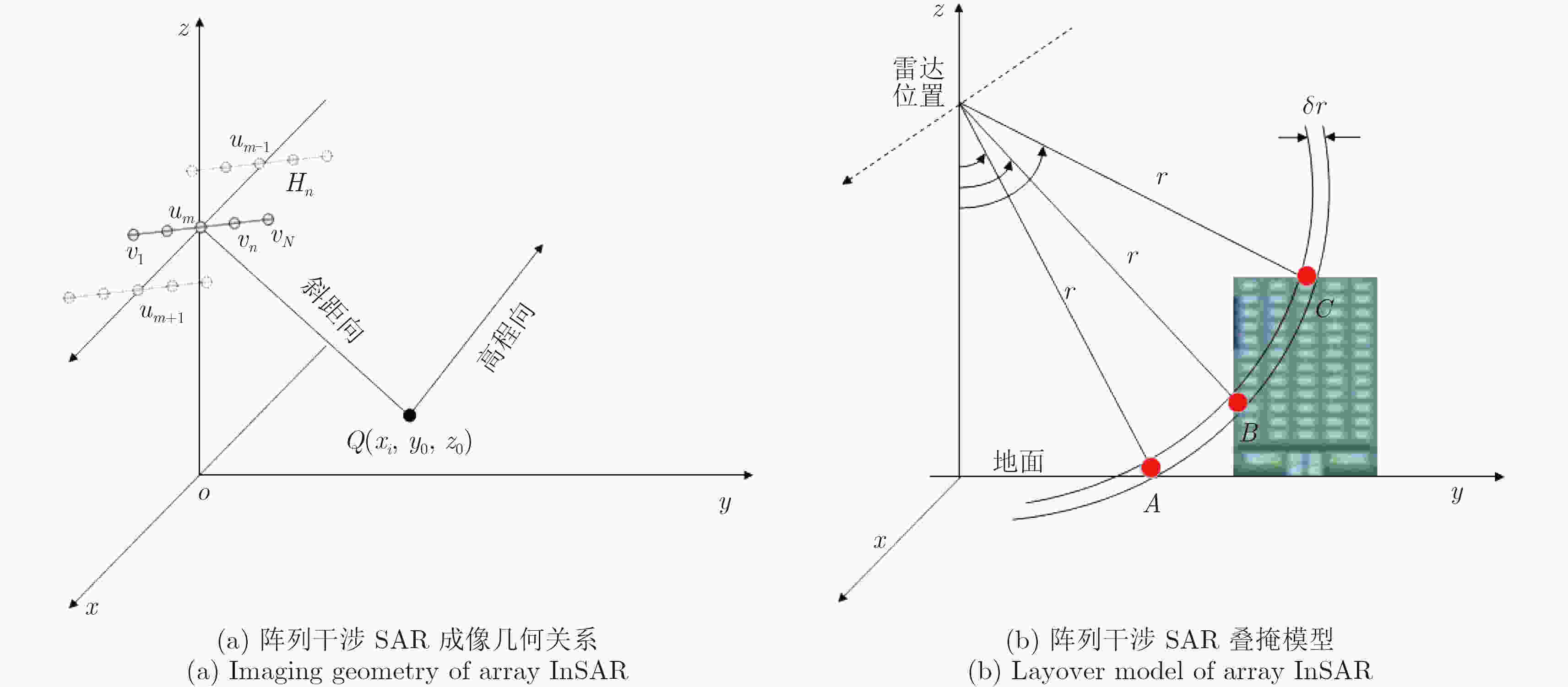
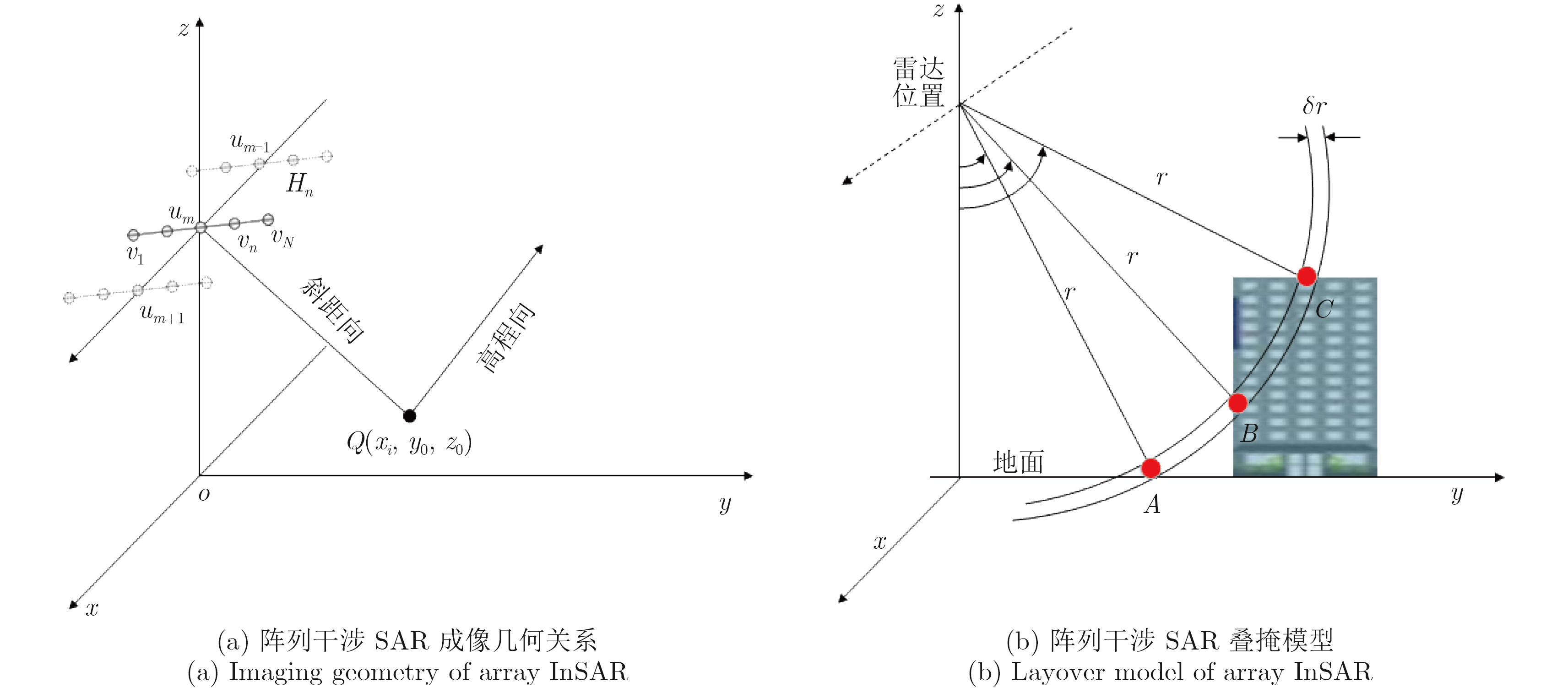
图 1 阵列干涉SAR成像模型

Figure 1. Array InSAR imaging model

下载: 全尺寸图片幻灯片

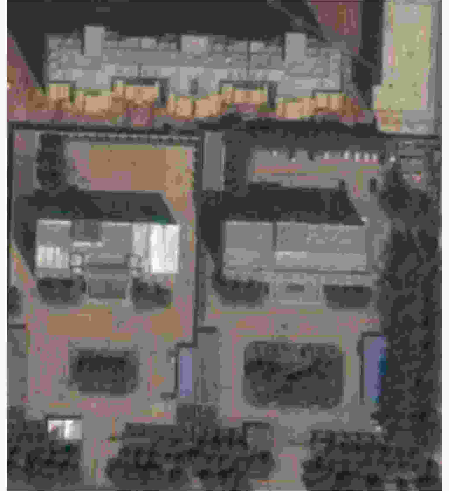
图 2 观测场景光学图像

Figure 2. Optical image of the observed scene

下载: 全尺寸图片幻灯片

图 3 观测场景原始3维点云

Figure 3. Orginal 3D point clouds of the observed scene

下载: 全尺寸图片幻灯片

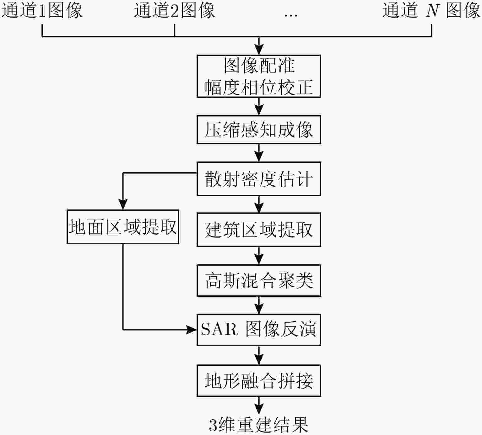
图 4 算法流程图

Figure 4. Workflow of proposed approach

下载: 全尺寸图片幻灯片

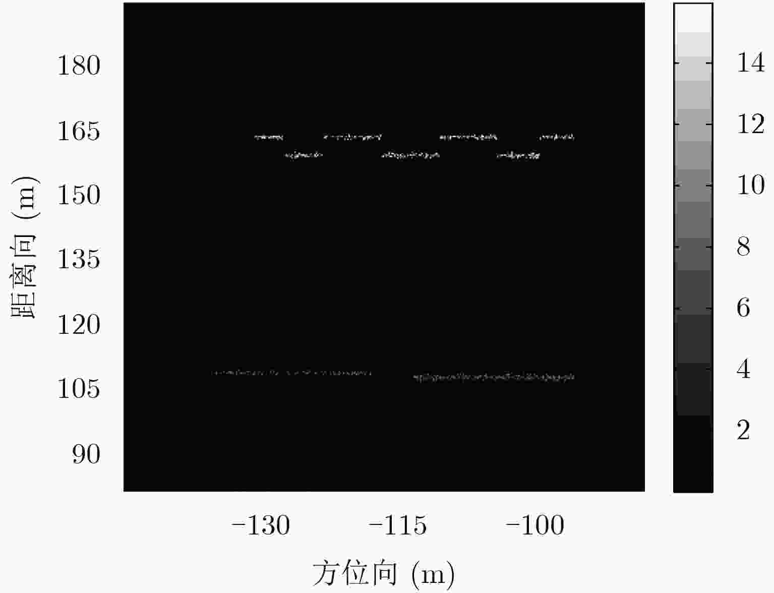
图 5 观测场景散射点密度图

Figure 5. Scatterer density map of the observed scene

下载: 全尺寸图片幻灯片

图 6 观测场景建筑物提取结果

Figure 6. Extracted building results of the observed scene

下载: 全尺寸图片幻灯片

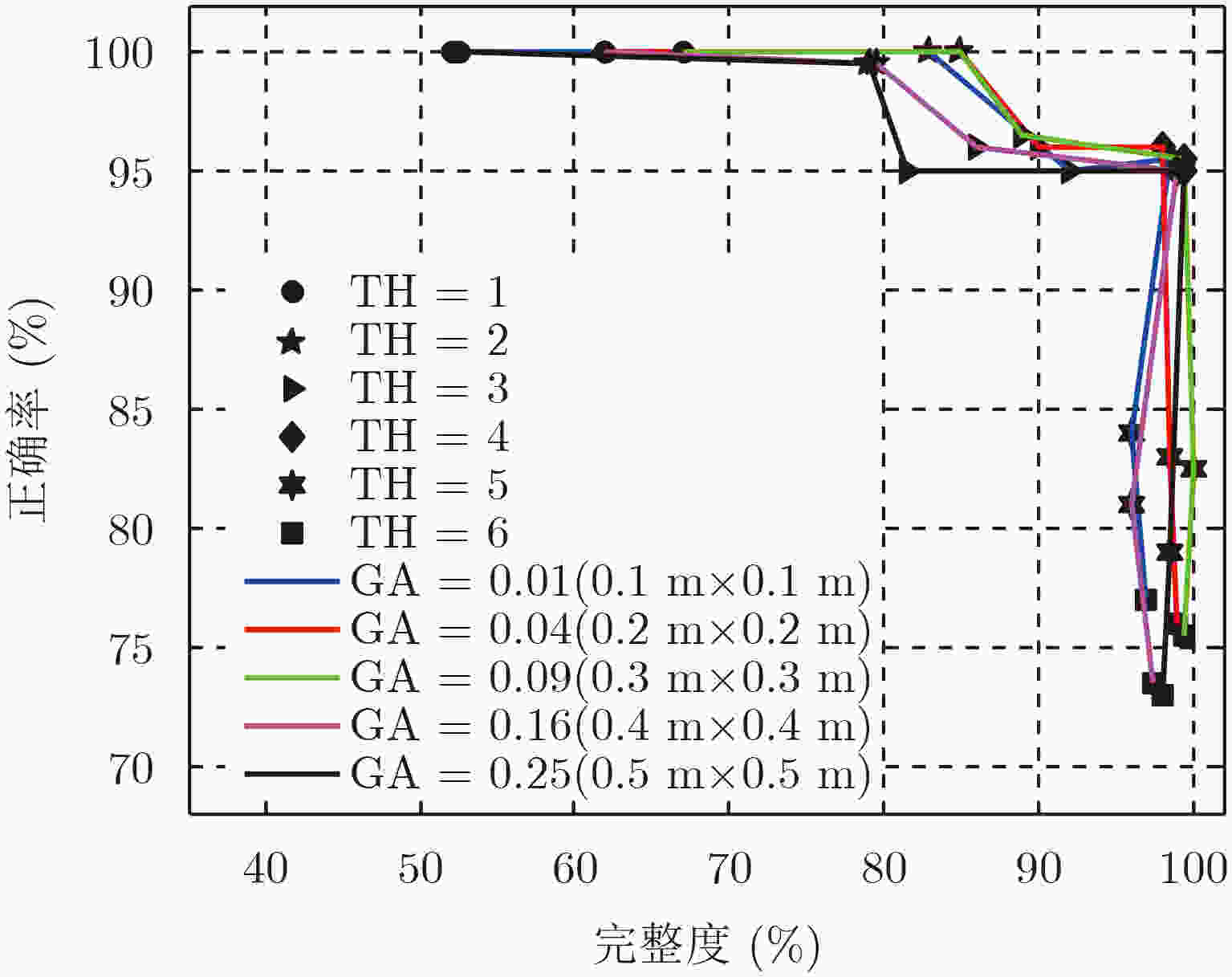
图 7 不同窗口/阈值性能曲线图

Figure 7. Performance curve map with varying TH and GA parameters

下载: 全尺寸图片幻灯片

图 8 子类个数与偏差度关系图

Figure 8. Dispersion plot with number of clusters

下载: 全尺寸图片幻灯片

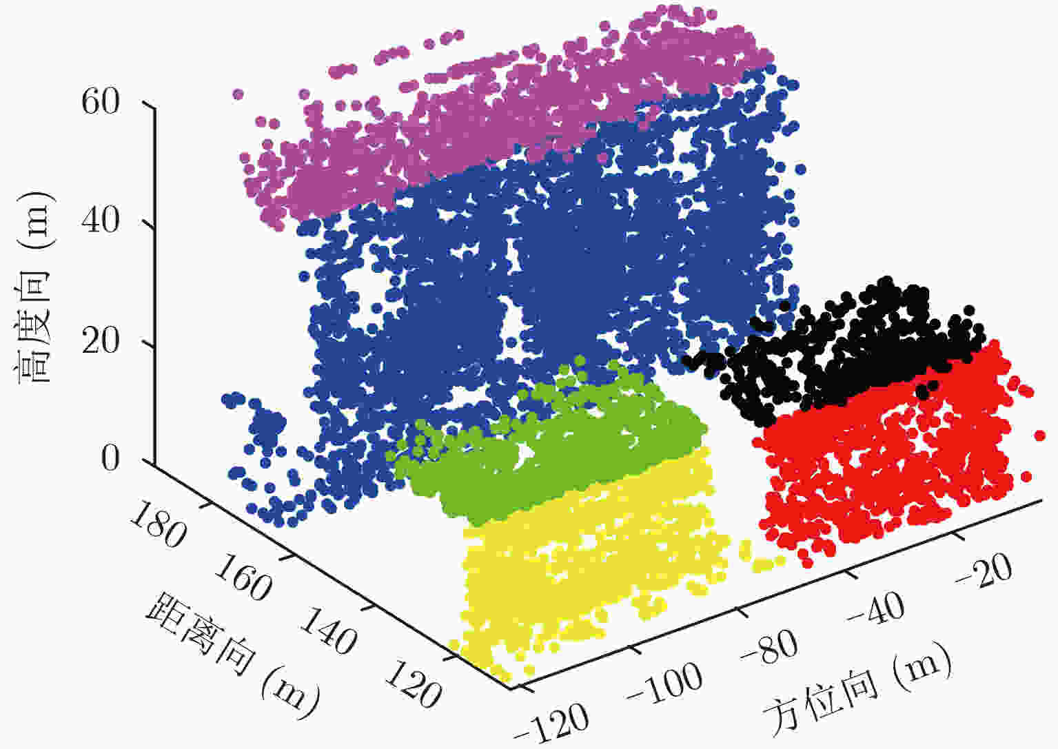
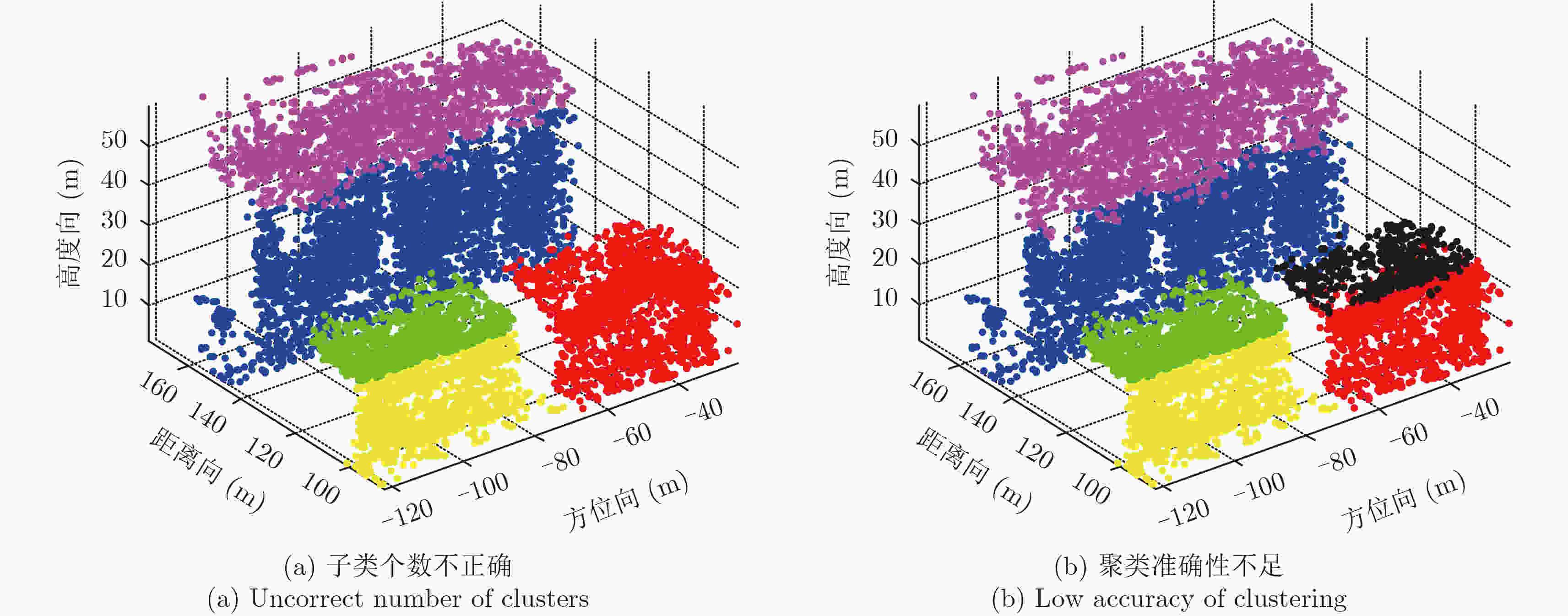
图 9 建筑物区域聚类结果

Figure 9. Clustered result of building areas

下载: 全尺寸图片幻灯片

图 10 K-means聚类结果

Figure 10. Clustered results of K-means

下载: 全尺寸图片幻灯片

图 11 各区域反演SAR图像

Figure 11. Inversed SAR images of all aeras

下载: 全尺寸图片幻灯片

图 12 地面区域SAR图像

Figure 12. Inversed SAR images of the ground

下载: 全尺寸图片幻灯片

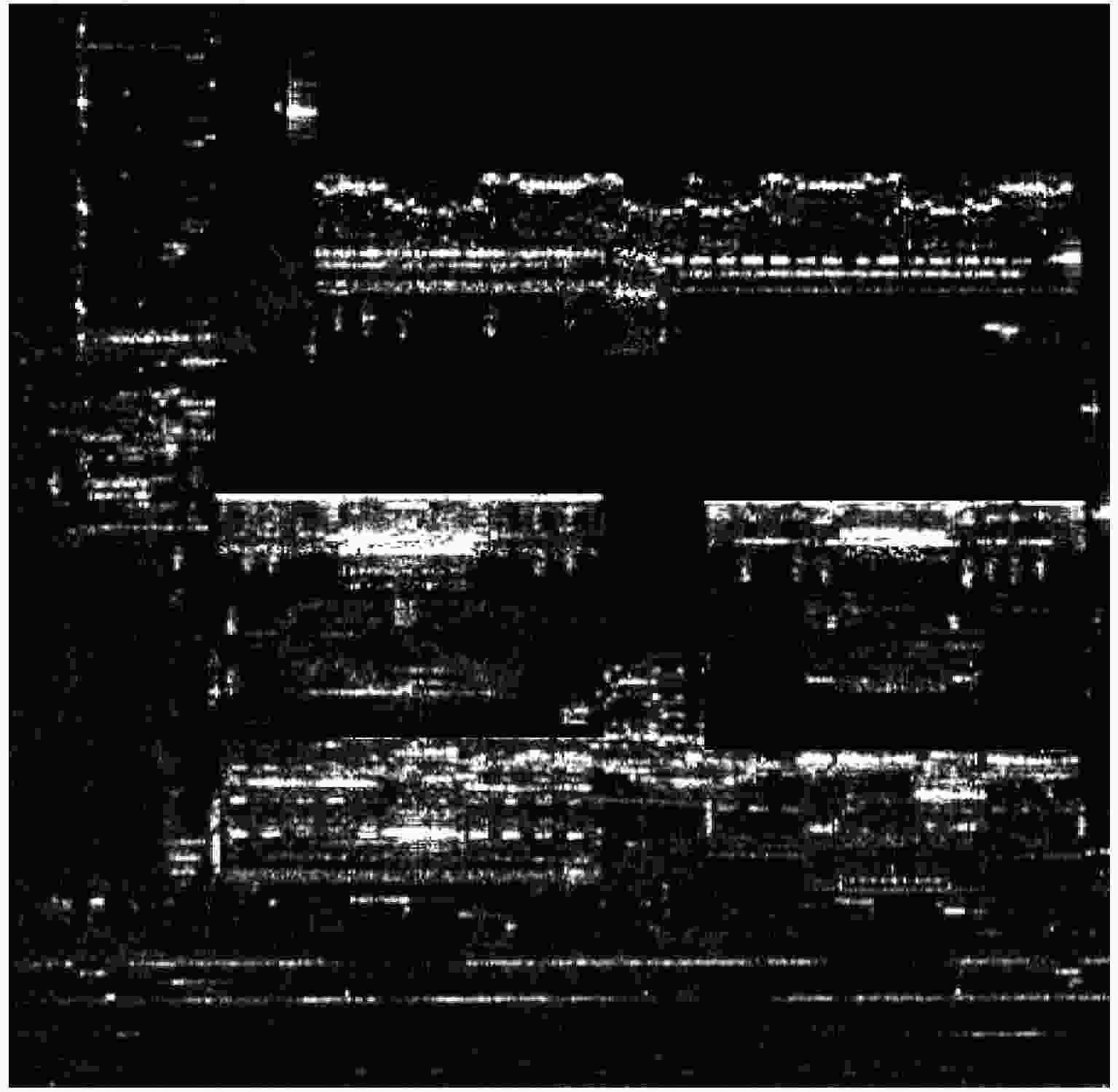
图 13 观测场景2维SAR图像

Figure 13. 2D SAR image of the observed scene

下载: 全尺寸图片幻灯片

图 14 观测场景干涉相位图

Figure 14. Interferometric phase image of the observed scene

下载: 全尺寸图片幻灯片

图 15 观测场景3维成像结果

Figure 15. 3D imaging result of the observed scene

下载: 全尺寸图片幻灯片

表 1 阵列干涉SAR系统参数

Table 1. System parameters of array InSAR

项目	参数
载频(GHz)	15
发射信号带宽(MHz)	500
脉冲重复频率(kHz)	1
载机高度(m)	600
飞行速度(m/s)	70
方位波束宽度(°)	2
距离波束宽度(°)	27
中心下视角(°)	25

下载: 导出CSV

表 2 不同窗口/阈值质量评价表

Table 2. Quality evaluation with varying TH and GA parameters

TH (点数/dm²)	GA (dm²)
TH (点数/dm²)	1×1	2×2	3×3	4×4	5×5
1	75.12	74.88	74.37	71.89	71.75
2	81.27	81.86	81.73	77.71	78.07
3	94.12	93.84	94.82	94.63	94.08
4	87.48	86.32	86.40	81.98	77.56
5	81.89	84.77	84.68	78.29	77.91
6	67.23	63.02	67.14	60.62	51.83

下载: 导出CSV

参考文献(20)

[1]	Morishita Y and Hanssen R F. Temporal decorrelation in L-, C-, and X-band satellite radar interferometry for pasture on drained peat soils[J]. IEEE Transactions on Geoscience and Remote Sensing, 2015, 53(2): 1096–1104. DOI: 10.1109/TGRS.2014.2333814.
[2]	张福博. 阵列干涉SAR三维重建信号处理技术研究[D]. [博士论文], 中国科学院大学, 2015. Zhang Fubo. Research on signal processing of 3-D reconstruction in linear array Synthetic Aperture Radar interferometry[D]. [Ph.D.dissertation], Institute of Electronics, Chinese Acedamy of Science, 2015.
[3]	Knaell K K and Cardillo G P. Radar tomography for the generation of three-dimensional images[J]. IEE Proceedings-Radar, Sonar and Navigation, 1995, 142(2): 54–60. DOI: 10.1049/ip-rsn:19951791.
[4]	Wang Bin, Wang Yanping, Hong Wen, et al.. Application of spatial spectrum estimation technique in multibaseline SAR for layover solution[C]. Proceedings of IEEE International Geoscience and Remote Sensing Symposium, Boston, USA, 2008: III-1139–III-1142.
[5]	王爱春, 向茂生. 基于块压缩感知的SAR层析成像方法[J]. 雷达学报, 2016, 5(1): 57–64. DOI: 10.12000/JR16006. Wang Aichun and Xiang Maosheng. SAR tomography based on block compressive sensing[J]. Journal of Radars, 2016, 5(1): 57–64. DOI: 10.12000/JR16006.
[6]	Reigber A and Moreira A. First demonstration of airborne SAR tomography using multibaseline L-band data[J]. IEEE Transactions on Geoscience and Remote Sensing, 2000, 38(5): 2142–2152. DOI: 10.1109/36.868873.
[7]	Zhu Xiaoxiang and Bamler R. Tomographic SAR inversion by L₁-norm regularization—the compressive sensing approach[J]. IEEE Transactions on Geoscience and Remote Sensing, 2010, 48(10): 3839–3846. DOI: 10.1109/TGRS.2010.2048117.
[8]	Zhu Xiaoxiang and Bamler R. Super-resolution power and robustness of compressive sensing for spectral estimation with application to spaceborne tomographic SAR[J]. IEEE Transactions on Geoscience and Remote Sensing, 2012, 50(1): 247–258. DOI: 10.1109/TGRS.2011.2160183.
[9]	Zivkovic Z. Improved adaptive Gaussian mixture model for background subtraction[C]. Proceedings of the 17th International Conference on Pattern Recognition, Cambridge, UK, 2004, 2: 28–31.
[10]	Budillon A, Evangelista A, and Schirinzi G. Three-dimensional SAR focusing from multipass signals using compressive sampling[J]. IEEE Transactions on Geoscience and Remote Sensing, 2011, 49(1): 488–499. DOI: 10.1109/TGRS.2010.2054099.
[11]	Donoho D L. Compressed sensing[J]. IEEE Transactions on Information Theory, 2006, 52(4): 1289–1306. DOI: 10.1109/TIT.2006.871582.
[12]	张福博, 梁兴东, 吴一戎. 一种基于地形驻点分割的多通道SAR三维重建方法[J]. 电子与信息学报, 2015, 37(10): 2287–2293. DOI: 10.11999/JEIT150244. Zhang Fu-bo, Liang Xing-dong, and Wu Yi-rong. 3-D reconstruction for multi-channel SAR interferometry using terrain stagnation point based division[J]. Journal of Electronics &Information Technology, 2015, 37(10): 2287–2293. DOI: 10.11999/JEIT150244.
[13]	廖明生, 魏恋欢, 汪紫芸, 等. 压缩感知在城区高分辨率SAR层析成像中的应用[J]. 雷达学报, 2015, 4(2): 123–129. DOI: 10.12000/JR15031. Liao Ming-sheng, Wei Lian-huan, Wang Zi-yun, et al. Compressive sensing in high-resolution 3D SAR tomography of urban scenarios[J]. Journal of Radars, 2015, 4(2): 123–129. DOI: 10.12000/JR15031.
[14]	Zhu Xiaoxiang and Shahzad M. Facade reconstruction using multiview spaceborne TomoSAR point clouds[J]. IEEE Transactions on Geoscience and Remote Sensing, 2014, 52(6): 3541–3552. DOI: 10.1109/TGRS.2013.2273619.
[15]	Sithole G and Vosselman G. Experimental comparison of filter algorithms for bare-Earth extraction from airborne laser scanning point clouds[J]. ISPRS Journal of Photogrammetry and Remote Sensing, 2004, 59(1-2): 85–101. DOI: 10.1016/j.isprsjprs.2004.05.004.
[16]	Vosselman G. Slope based filtering of laser altimetry data[J]. International Archives of Photogrammetry and Remote Sensing, 2000, 33(B3/2), Part 3: 935–942.
[17]	Rottensteiner F and Briese C. A new method for building extraction in urban areas from high-resolution LIDAR data[J]. International Archives of Photogrammetry Remote Sensing and Spatial Information Sciences, 2002, 34(3/A): 295–301.
[18]	Vrieze S I. Model selection and psychological theory: A discussion of the differences between the Akaike information criterion (AIC) and the Bayesian information criterion (BIC)[J]. Psychological Methods, 2012, 17(2): 228–243. DOI: 10.1037/a0027127.
[19]	Moon T K. The expectation-maximization algorithm[J]. IEEE Signal Processing Magazine, 1996, 13(6): 47–60. DOI: 10.1109/79.543975.
[20]	Sampath A and Shan Jie. Segmentation and reconstruction of polyhedral building roofs from aerial lidar point clouds[J]. IEEE Transactions on Geoscience and Remote Sensing, 2010, 48(3): 1554–1567. DOI: 10.1109/TGRS.2009.2030180.

施引文献

期刊类型引用(5)

1.	布锦钶，李鹏飞，周鹏，周志一，曾祥祝，胡城志，孙兴赛，赵青，张文理. 基于杂波知识图谱驱动的空时自适应处理方法. 物联网技术. 2024(11): 122-126 . 百度学术
2.	陈慧，田湘，王文钦. 共形FDA-MIMO波束图综合. 信号处理. 2023(05): 793-806 . 百度学术
3.	胡瑞贤，贾秀权，曹晨. 基于频控阵波束锐化的主瓣干扰抑制技术. 中国电子科学研究院学报. 2023(08): 770-778 . 百度学术
4.	兰岚，廖桂生，许京伟，朱圣棋，曾操，张玉洪. 基于频率分集阵列的多功能一体化波形设计与信号处理方法. 雷达学报. 2022(05): 850-870 . 本站查看
5.	王文钦，张顺生. 频控阵雷达技术研究进展综述. 雷达学报. 2022(05): 830-849 . 本站查看

其他类型引用(3)

资源附件(0)

访问统计

图(15) / 表(2)

计量

文章访问数: 3069
HTML全文浏览量: 680
PDF下载量: 576
被引次数: 8

1. Introduction
2. Conformal FDA-MIMO Radar
2.1 General conformal FDA-MIMO signal model
2.2 CRLB of conformal FDA-MIMO
3. Reduced-Dimension Target Parameter Estimation Algorithm
4. Simulation Results
4.1 Analysis of computational complexity
4.2 Single target parameter estimation
4.3 Multiple targets parameter estimation
5. Conclusion

1. Introduction
2. Conformal FDA-MIMO Radar
2.1 General conformal FDA-MIMO signal model
2.2 CRLB of conformal FDA-MIMO
3. Reduced-Dimension Target Parameter Estimation Algorithm
4. Simulation Results
4.1 Analysis of computational complexity
4.2 Single target parameter estimation
4.3 Multiple targets parameter estimation
5. Conclusion

参考文献(20)

施引文献

资源附件(0)

访问统计

基于高斯混合聚类的阵列干涉SAR三维成像

DOI: 10.12000/JR17020

通讯作者:
梁兴东 xdliang@mail.ie.ac.cn

计量

3D Imaging for Array InSAR Based on Gaussian Mixture Model Clustering

1. Introduction

2. Conformal FDA-MIMO Radar

2.1 General conformal FDA-MIMO signal model

2.2 CRLB of conformal FDA-MIMO

3. Reduced-Dimension Target Parameter Estimation Algorithm

4. Simulation Results

4.1 Analysis of computational complexity

4.2 Single target parameter estimation

4.3 Multiple targets parameter estimation

5. Conclusion

期刊类型引用(5)

其他类型引用(3)

计量

目录

1. Introduction

2. Conformal FDA-MIMO Radar

2.1 General conformal FDA-MIMO signal model

2.2 CRLB of conformal FDA-MIMO

3. Reduced-Dimension Target Parameter Estimation Algorithm

4. Simulation Results

4.1 Analysis of computational complexity

4.2 Single target parameter estimation

4.3 Multiple targets parameter estimation

5. Conclusion

期刊介绍

联系我们

基于高斯混合聚类的阵列干涉SAR三维成像

DOI: 10.12000/JR17020

通讯作者: 梁兴东 xdliang@mail.ie.ac.cn

计量

出版历程

3D Imaging for Array InSAR Based on Gaussian Mixture Model Clustering

1. Introduction

2. Conformal FDA-MIMO Radar

2.1 General conformal FDA-MIMO signal model

2.2 CRLB of conformal FDA-MIMO

3. Reduced-Dimension Target Parameter Estimation Algorithm

4. Simulation Results

4.1 Analysis of computational complexity

4.2 Single target parameter estimation

4.3 Multiple targets parameter estimation

5. Conclusion

期刊类型引用(5)

其他类型引用(3)

计量

出版历程

目录

1. Introduction

2. Conformal FDA-MIMO Radar

2.1 General conformal FDA-MIMO signal model

2.2 CRLB of conformal FDA-MIMO

3. Reduced-Dimension Target Parameter Estimation Algorithm

4. Simulation Results

4.1 Analysis of computational complexity

4.2 Single target parameter estimation

4.3 Multiple targets parameter estimation

5. Conclusion

期刊介绍

联系我们

通讯作者:
梁兴东 xdliang@mail.ie.ac.cn