
 Submit Manuscript
 Peer Review
 Editor Work
- Home
- Articles & Issues
-
Data
- Dataset of Radar Detecting Sea
- SAR Dataset
- SARGroundObjectsTypes
- SARMV3D
- AIRSAT Constellation SAR Land Cover Classification Dataset
- 3DRIED
- UWB-HA4D
- LLS-LFMCWR
- FAIR-CSAR
- MSAR
- SDD-SAR
- FUSAR
- SpaceborneSAR3Dimaging
- Sea-land Segmentation
- SAR Multi-domain Ship Detection Dataset
- SAR-Airport
- Hilly and mountainous farmland time-series SAR and ground quadrat dataset
- SAR images for interference detection and suppression
- HP-SAR Evaluation & Analytical Dataset
- GDHuiYan-ATRNet
- Multi-System Maritime Low Observable Target Dataset
- DatasetinthePaper
- DatasetintheCompetition
- Report
- Course
- About
- Publish
- Editorial Board
- Chinese
| Citation: | Zhou Yang, Bi Daping, Shen Aiguo, Fang Mingxing. Intermittent Sampling Repeater Shading Jamming Method Based on Motion Modulation for SAR-GMTI[J]. Journal of Radars, 2017, 6(4): 359-367. doi: 10.12000/JR16075

|
Intermittent Sampling Repeater Shading Jamming Method Based on Motion Modulation for SAR-GMTI
DOI: 10.12000/JR16075 CSTR: 32380.14.JR16075
-
Abstract
In this paper, we present a shading jamming method for the Synthetic Aperture Radar and Ground Moving Target Indicator (SAR-GMTI). This method begins with intermittently sampling intercepted SAR signals, performing motion modulation, and then transmitting them. The motion modulation of SAR signals can produce a motion modulation effect and intermittent sampling repeater jamming can produce multi-fronted and lagged false targets along a range. Their combination provides a jamming effect of smart shading areas, which can’t be cancelled after multi-channel cancelling. The uniqueness of this jamming method is that the energy only appears on the moving target to be covered, so less jamming energy is needed. We analyzed the proposed jamming principle against GMTI using the tri-channel interference cancelling technique. Our simulation results verify our analyses and confirm its jamming effectiveness for SAR-GMTI. -

-
References
[1] Zhang Xue-pan, Liao Gui-sheng, Zhu Sheng-qi, et al. Geometry-information-aided efficient motion parameter estimation for moving-target imaging and location[J]. IEEE Geoscience and Remote Sensing Letters, 2015, 12(1): 155–159. DOI: 10.1109/LGRS.2014.2329941[2] Huang Long, Dong Chun-xi, Shen Zhi-bo, et al. The influence of rebound jamming on SAR GMTI[J]. IEEE Geoscience and Remote Sensing Letters, 2015, 12(2): 399–403. DOI: 10.1109/LGRS.2014.2345091[3] Zhang Shuang-xi, Xing Meng-dao, Xia Xiang-gen, et al. Robust clutter suppression and moving target imaging approach for multichannel in azimuth high-resolution and wide-swath synthetic aperture radar[J]. IEEE Transactions on Geoscience and Remote Sensing, 2015, 53(2): 687–709. DOI: 10.1109/TGRS.2014.2327031[4] 李兵, 洪文. 合成孔径雷达噪声干扰研究[J]. 电子学报, 2005, 32(12): 2035–2037Li Bing and Hong Wen. Study of noise jamming to SAR[J]. Acta Electronica Sinica, 2005, 32(12): 2035–2037[5] 蔡幸福, 宋建社, 郑永安, 等. 二维间歇采样延迟转发SAR干扰技术及其应用[J]. 系统工程与电子技术, 2015, 37(3): 566–571Cai Xing-fu, Song Jian-she, Zheng Yong-an, et al. SAR jamming technology based on 2-D intermittent sampling delay repeater and its application[J]. Systems Engineering and Electronics, 2015, 37(3): 566–571[6] 黄龙, 董春曦, 赵国庆. 利用多干扰机对抗SAR双通道干扰对消技术的研究[J]. 电子与信息学报, 2014, 36(4): 904–907Huang Long, Dong Chun-xi, and Zhao Guo-qing. Investigation on countermeasure against SAR dual-channel cancellation technique with multi-jammers[J]. Journal of Electronics&Information Technology, 2014, 36(4): 904–907[7] 黄龙, 董春曦, 沈志博, 等. 多天线干扰机对抗InSAR双通道干扰对消的研究[J]. 电子与信息学报, 2015, 37(4): 913–918 doi: 10.11999/JEIT140769Huang Long, Dong Chun-xi, Shen Zhi-bo, et al. Investigation on countermeasure against InSAR dual-channel cancellation technique with multi-antenna jammer[J]. Journal of Electronics&Information Technology, 2015, 37(4): 913–918. DOI: 10.11999/JEIT140769[8] 吴晓芳, 王雪松, 梁景修. SAR-GMTI高逼真匀速运动假目标调制干扰方法[J]. 宇航学报, 2012, 33(10): 1472–1479 doi: 10.3873/j.issn.1000-1328.2012.10.016Wu Xiao-fang, Wang Xue-song, and Liang Jing-xiu. Modulation jamming method for high-vivid false uniformly-moving targets against SAR-GMTI[J].Journal of Astronautics, 2012, 33(10): 1472–1479. DOI: 10.3873/j.issn.1000-1328.2012.10.016[9] 吴晓芳, 梁景修, 王雪松, 等. SAR-GMTI匀加速运动假目标有源调制干扰方法[J]. 宇航学报, 2012, 33(6): 761–768Wu Xiao-fang, Liang Jing-xiu, Wang Xue-song, et al. Modulation jamming method of active false uniformly-accelerating targets against SAR-GMTI[J]. Journal of Astronautics, 2012, 33(6): 761–768[10] 王雪松, 刘建成, 张文明, 等. 间歇采样转发干扰的数学原理[J]. 中国科学E辑: 信息科学, 2006, 36(8): 891–901Wang Xue-song, Liu Jian-cheng, Zhang Wen-ming, et al. Mathematical principles of intermittent sampling repeater jamming[J]. Science in China Series E:Information Sciences, 2006, 36(8): 891–901[11] 孙光才, 周峰, 邢孟道. 一种SAR-GMTI的无源压制性干扰方法[J]. 系统工程与电子技术, 2010, 32(1): 39–45Sun Guang-cai, Zhou Feng, and Xing Meng-dao. New passive barrage jamming method for SAR-GMTI[J]. Systems Engineering and Electronics, 2010, 32(1): 39–45[12] 周阳, 房明星, 毕大平, 等. 旋转角反射器阵列对SAR-GMTI的无源遮蔽干扰方法[J]. 探测与控制学报, 2017, 39(2): 87–93Zhou Yang, Fang Ming-xing, Bi Da-ping, et al. A passive shading jamming method to SAR-GMTI using array rotating angular reflectors[J]. Journal of Detection&Control, 2017, 39(2): 87–93[13] 吴晓芳, 王雪松, 卢焕章. 对SAR的间歇采样转发干扰研究[J]. 宇航学报, 2009, 30(5): 2043–2049Wu Xiao-fang, Wang Xue-song, and Lu Huan-zhang. Study of intermittent sampling repeater jamming to SAR[J]. Journal of Astronautics, 2009, 30(5): 2043–2049[14] Sjögren T K, Vu V T, Pettersson M I, et al. Suppression of clutter in multichannel SAR GMTI[J]. IEEE Transactions on Geoscience and Remote Sensing, 2014, 52(7): 4005–4013. DOI: 10.1109/TGRS.2013.2278701[15] 周阳, 毕大平, 房明星, 等. 对SAR-GMTI的运动调制-步进移频复合干扰[J]. 信号处理, 2016, 32(12): 1468–1477Zhou Yang, Bi Da-ping, Fang Ming-xing, et al. A motion modulated and step frequency shifting compound interference to SAR-GMTI[J]. Journal of Signal Processing, 2016, 32(12): 1468–1477 -
Proportional views

- Publishing Ethics
- Journal Insights
- Abstracting & Indexing
- Peer Review Policies
- Guide for Authors
- Conference
- ISSN 2095-283X (Print)ISSN 2097-339X (Online)
- CN 10-1030/TN
- CODEN LXEUAO
About Journal
- Sponsor: China Radio Detection and Ranging Industry Association (CRIA)
- Phone: 010-58887062
- Email:radars@aircas.ac.cn
- Publisher: Leida Xuebao Bianjibu (Editorial office of the Journal of Radars)
Contacts Us

京ICP备20021838号-14
Supported by: Beijing Renhe Information Technology Co. Ltd

Export File
Citation
Format
Content
 DownLoad:


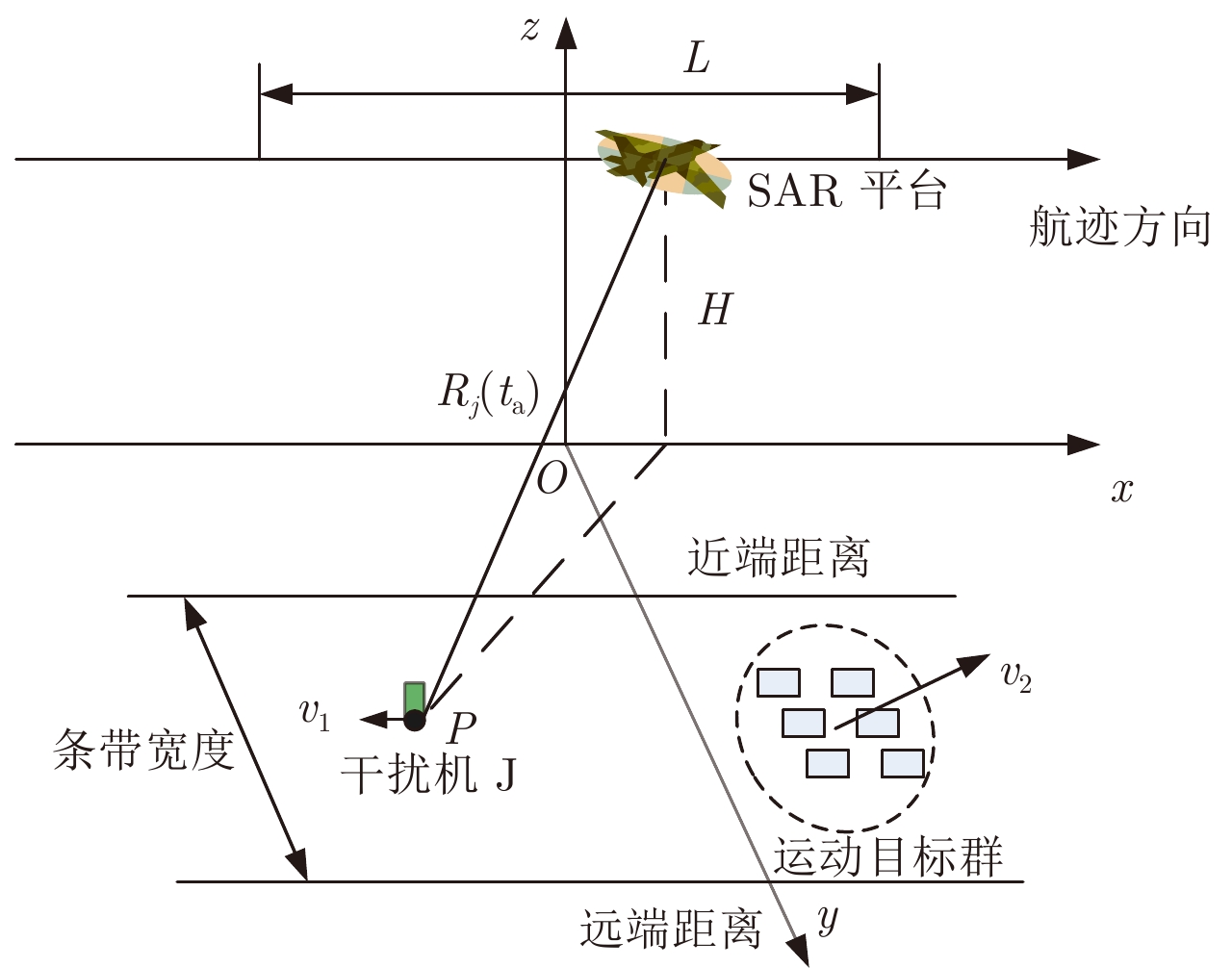
- Figure 1. The imaging scene of SAR
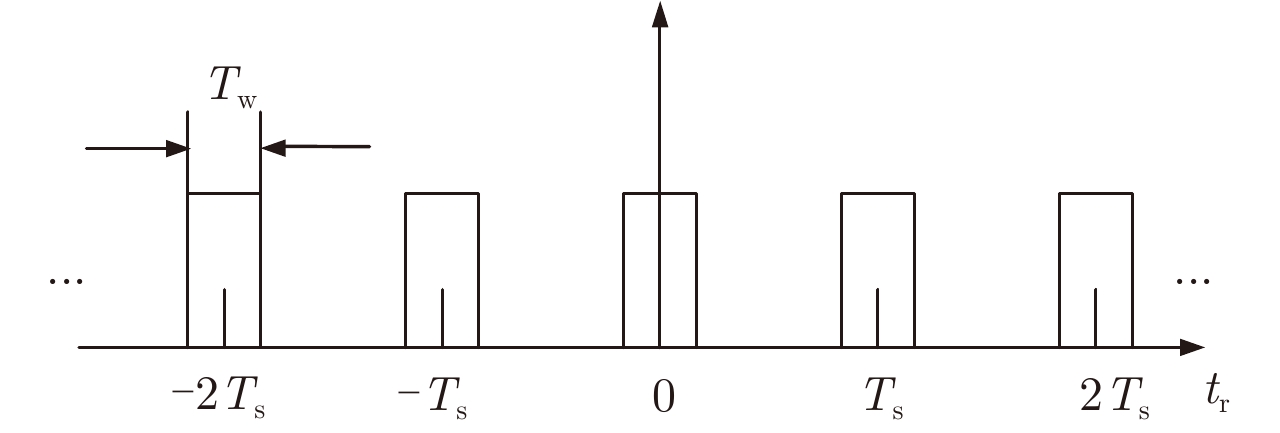
- Figure 2. Azimuth intermittent sampling pulse series
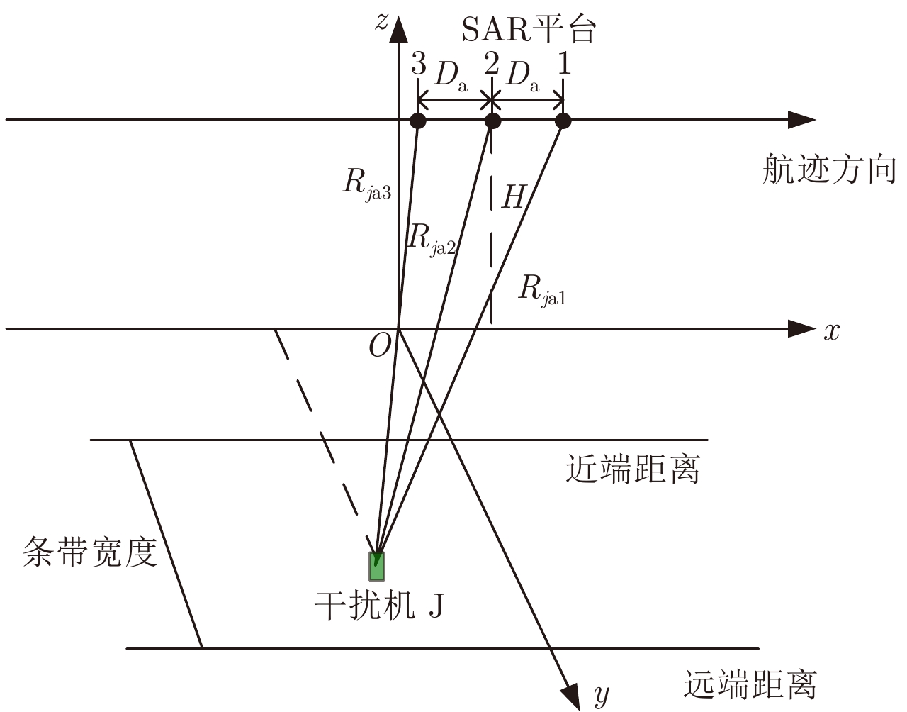
- Figure 3. The sketch map of tri-antenna interference cancelling technique
- Figure 4. The jamming images effect of shading six armored car
- Figure 5. Jamming images with different sampling periods
- Figure 6. Jamming images with different duty ratio
- Figure 7. Jamming images with different motion modulation parameters