基于多传感器融合的协同感知方法

王秉路; 靳杨; 张磊; 郑乐; 周天飞

doi:10.12000/JR23184

基于多传感器融合的协同感知方法

DOI: 10.12000/JR23184

王秉路^{1, 2},
靳杨¹,
张磊³,
郑乐²,
周天飞^4, ,

1.
西安建筑科技大学信息与控制工程学院西安 710399
2.
北京理工大学信息与电子学院北京 100081
3.
西北工业大学自动化学院西安 710129
4.
北京理工大学计算机学院北京 100081

基金项目: 中国博士后科学基金(2022M710393, 2022TQ0035)

详细信息

作者简介:
王秉路，博士，副教授，主要研究方向为多模态信息融合

靳　杨，硕士生，主要研究方向为计算机视觉和深度学习

张　磊，博士生，主要研究方向为计算机视觉和深度学习

郑　乐，博士，教授，主要研究方向为雷达目标跟踪和雷达成像

周天飞，博士，教授，主要研究方向为图像处理、深度学习和机器学习

通讯作者:
周天飞 ztfei.debug@gmail.com

责任主编：刘凡 Corresponding Editor: LIU Fan
中图分类号: TN957.51
计量
- 文章访问数: 2911
- HTML全文浏览量: 289
- PDF下载量: 621
- 被引次数: 10
出版历程
- 收稿日期: 2023-10-04
- 修回日期: 2023-12-10
- 网络出版日期: 2023-12-27
- 刊出日期: 2024-02-28

Collaborative Perception Method Based on Multisensor Fusion

WANG Binglu^{1, 2},
JIN Yang¹,
ZHANG Lei³,
ZHENG Le²,
ZHOU Tianfei^{4
, ,}

1.
College of Information and Control Engineering, Xi’an University of Architecture and Technology, Xi’an 710399, China
2.
School of Information and Electronics, Beijing Institute of Technology, Beijing 100081, China
3.
School of Automation, Northwestern Polytechnical University, Xi’an 710129, China
4.
School of Computer Science & Technology, Beijing Institute of Technology, Beijing 100081, China

Funds: China Postdoctoral Science Foundation (2022M710393, 2022TQ0035)

More Information

Corresponding author: ZHOU Tianfei, ztfei.debug@gmail.com

摘要

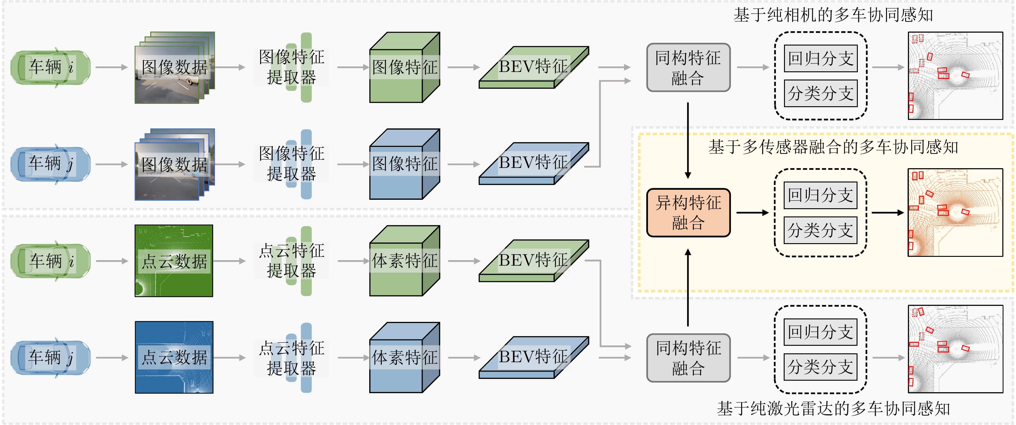
摘要: 该文提出了一种新的多模态协同感知框架，通过融合激光雷达和相机传感器的输入来增强自动驾驶感知系统的性能。首先，构建了一个多模态融合的基线系统，能有效地整合来自激光雷达和相机传感器的数据，为后续研究提供了可比较的基准。其次，在多车协同环境下，探索了多种流行的特征融合策略，包括通道级拼接、元素级求和，以及基于Transformer的融合方法，以此来融合来自不同类型传感器的特征并评估它们对模型性能的影响。最后，使用大规模公开仿真数据集OPV2V进行了一系列实验和评估。实验结果表明，基于注意力机制的多模态融合方法在协同感知任务中展现出更优越的性能和更强的鲁棒性，能够提供更精确的目标检测结果，从而增加了自动驾驶系统的安全性和可靠性。
- 自动驾驶 /
- 协同感知 /
- 3D目标检测 /
- 多模态融合 /
- 智能交通系统
Abstract: This paper proposes a novel multimodal collaborative perception framework to enhance the situational awareness of autonomous vehicles. First, a multimodal fusion baseline system is built that effectively integrates Light Detection and Ranging (LiDAR) point clouds and camera images. This system provides a comparable benchmark for subsequent research. Second, various well-known feature fusion strategies are investigated in the context of collaborative scenarios, including channel-wise concatenation, element-wise summation, and transformer-based methods. This study aims to seamlessly integrate intermediate representations from different sensor modalities, facilitating an exhaustive assessment of their effects on model performance. Extensive experiments were conducted on a large-scale open-source simulation dataset, i.e., OPV2V. The results showed that attention-based multimodal fusion outperforms alternative solutions, delivering more precise target localization during complex traffic scenarios, thereby enhancing the safety and reliability of autonomous driving systems.
- Autonomous driving /
- Collaborative perception /
- 3D object detection /
- Multimodal fusion /
- Intelligent transportation systems

HTML全文

1. Introduction

In recent years, Frequency Diverse Array (FDA) radar has received much attention due to its range-angle-time-dependent beampattern^[1,2]. Combining the advantages of FDA and traditional phased array Multiple-Input Multiple-Output (MIMO) radar in the degree of freedom, the FDA Multiple-Input Multiple Output (FDA-MIMO) radar was proposed in Ref. [3] and applied in many fields^[4-9]. For parameter estimation algorithm, the authors first proposed a FDA-MIMO target localization algorithm based on sparse reconstruction theory^[10], and an unbiased joint range and angle estimation method was proposed in Ref. [11]. The work of Ref. [12] further proved that the FDA-MIMO is superior to traditional MIMO radar in range and angle estimation performance, and the authors of Ref. [13] introduced a super-resolution MUSIC algorithm for target location, and analyzed its resolution threshold. Meanwhile, high-resolution Doppler processing is utilized for moving target parameter estimation^[14]. The Estimation of Signal Parameters via Rotational Invariance Technique (ESPRIT) and PARAllel FACtor (PARAFAC) was proposed in Ref. [15], which is a search-free algorithm for FDA-MIMO.

Moreover, the research of conformal array has received more and more attention. Conformal array is a non-planar array that can be completely attached to the surface of the carrier^[16]. It has significant advantages such as reducing the aerodynamic impact on the carrier and smaller radar cross section^[17]. In addition, conformal array can achieve wide-angle scanning with a lower SideLobe Level (SLL)^[18]. Different from traditional arrays, the element beampattern of conformal array needs to be modeled separately in the parameter estimation due to the difference of carrier curvature^[19-21].

As far as we know, most of the existing researches on FDA-MIMO are based on linear array, while there is little research on the combination of FDA-MIMO and conformal array^[22]. In this paper, we replace the receiving array in the traditional FDA-MIMO with conformal array. Compared with conventional FDA-MIMO, conformal FDA-MIMO inherits the merits of conformal array and FDA-MIMO, which can effectively improve the stealth and anti-stealth performance of the carrier, and reduce the volume and the air resistance of the carrier. For conformal FDA-MIMO, we further study the parameters estimation algorithm. The major contributions of this paper are summarized as follows:

(1) A conformal FDA-MIMO radar model is first formulated.

(2) The parameter estimation Cramér-Rao Lower Bound (CRLB) for conformal FDA-MIMO radar is derived.

(3) Inspired by the existing work of Refs. [23,24], a Reduced-Dimension MUSIC (RD-MUSIC) algorithm for conformal FDA-MIMO radar is correspondingly proposed to reduce the complexity.

The rest of the paper consists of four parts. Section 2 formulates the conformal FDA-MIMO radar model, and Section 3 derives a RD-MUSIC algorithm for conformal FDA-MIMO radar. Simulation results for conformal FDA-MIMO radar with semi conical conformal receiving array are provided in Section 4. Finally, conclusions are drawn in Section 5.

2. Conformal FDA-MIMO Radar

2.1 General conformal FDA-MIMO signal model

For the convenience of analysis, we consider a monostatic conformal FDA-MIMO radar which is composed by a $M$ -element linear FDA transmitting array and a $N$ -element conformal receiving array, as shown in Fig. 1. d denotes the inter-element spacing, the carrier frequency at the mth transmitting element is ${f_m} = {f_1} + \Delta f(m - 1)$ , $m = 1,2, \cdots ,M$ where ${f_1}$ is the transmission frequency of the first antenna element, which is called as reference frequency, and $\Delta f$ is the frequency offset between the adjacent array elements.

Figure 1. Conformal FDA-MIMO radar

DownLoad: Full-Size Img PowerPoint

The complex envelope of the transmitted signal of the mth transmitting element is denoted as ${{\varphi _m}} (t)$ , assume the transmitting waveforms have orthogonality,

$\int_{{T_p}} {{\varphi _m}} (t)\varphi _{{m_1}}^*(t - \tau ){\rm{d}}t = 0,\quad {m_1} \ne m$

(1)

where $\tau$ denotes the time delay, ${T_p}$ denotes the pulse duration, and ${\left( \cdot \right)^ * }$ is conjugate operator. The signal transmitted from the mth element can be expressed as

${s_m}(t) = {a_m}(t,\theta ,\phi ,r){\varphi _m}(t),\quad 0 \le t \le {T_p}$

(2)

where

$\begin{split} & {a_m}(t,\theta ,\phi ,r) \hfill \\ & =\exp \left\{ { - {\rm{j}}2\pi \left( \begin{gathered} \frac{{(m - 1)\Delta fr}}{{\rm{c}}} - \frac{{{f_1}(m - 1){{d}}\sin \alpha }}{{\rm{c}}} \hfill \\ - (m - 1)\Delta ft \hfill \\ \end{gathered} \right)} \right\} \end{split}$

(3)

is the mth element of the transmitting steering vector according to the phase difference between adjacent elements, the angle between far-field target and transmitting array is denoted as $\alpha = \arcsin (\sin \theta \cos \phi )$ , where $\arcsin ( \cdot )$ denotes arcsine operator, $\alpha$ can be calculated by using the inner product between the target vector and unit vector along the $X$ -axis. $\theta ,\phi ,r$ are the elevation, azimuth and range between the target and the origin point, respectively. The phase difference between adjacent elements is

$\Delta {\psi _{t0}} = 2\pi \left( {\frac{{\Delta fr}}{{\rm{c}}} - \frac{{{f_1}d\sin \alpha }}{{\rm{c}}} - \Delta ft} \right)$

(4)

where ${\rm{c}}$ is light speed. For far-field target ${P}\left( {r,\theta ,\phi } \right)$ , the transmitting steering vector is

$\begin{split} {{\boldsymbol{a}}_0}\left( {t,\theta ,\phi ,r} \right) =& \left[ {1,\exp \left\{ { - {\rm{j}}\Delta {\psi _{t0}}} \right\}, \cdots ,} \right. \\ &{\left. {\exp \left\{ { - {\rm{j}}(M - 1)\Delta {\psi _{t0}}} \right\}} \right]^{\rm{T}}} \end{split}$

(5)

For the conformal receiving array, as shown in Fig. 1(b), the time delay between target ${P}\left( {r,\theta ,\phi } \right)$ and the nth receiving array element is

${\tau _n} = {r_n}/{\rm{c}}$

(6)

where ${r_n}$ is the range between target and the nth receiving array element. For far-field assumption, the ${r_n}$ can be approximated as

${r_n} \approx r - {\vec {\boldsymbol{p}}_n} \cdot \vec {\boldsymbol{r}}$

(7)

where r denotes the range between the target and the origin point, ${\vec {\boldsymbol{p}}_n} = {x_n}{{\boldsymbol{e}}_x} + {y_n}{{\boldsymbol{e}}_y} + {z_n}{{\boldsymbol{e}}_z}$ denotes the position vector from the nth element to origin point, and $\vec {\boldsymbol{r}} = \sin \theta \cos \phi {{\boldsymbol{e}}_x} + \sin \theta \sin \phi {{\boldsymbol{e}}_y} + \cos\theta {{\boldsymbol{e}}_z}$ is the unit vector in target orientation, where ${{\boldsymbol{e}}_x},{{\boldsymbol{e}}_y}$ and ${{\boldsymbol{e}}_z}$ are the unit vectors along the X- , Y- , and $Z$ -axis, respectively. $({x_n},{y_n},{z_n})$ are the coordinates of the nth element in the Cartesian coordinate system. For simplicity, we let $u = \sin \theta \cos \phi$ , $v = \sin \theta \cos \phi$ , so the time delay ${\tau _n} =$ $(r - (u{x_n} + v{y_n} + \cos \theta {z_n}))/{\rm{c}}$ . The time delay between the first element and the nth element at the receiving array is expressed as

$\begin{split} \Delta {\tau _{{r_n}}} =& {\tau _1} - {\tau _n} \\ =& \frac{{u({x_n} - {x_1}) + v({y_n} - {y_1}) + \cos \theta ({z_n} - {z_1})}}{{\rm{c}}} \\ \end{split}$

(8)

And the corresponding phase difference between the first element and the nth element is

$\Delta {\psi _{{R_n}}} = 2\pi {f_1}\Delta {\tau _{{r_n}}}$

(9)

Consequently, the receiving steering vector is

$\begin{split} {\boldsymbol{b}}\left( {\theta ,\phi } \right) =& \left[ {{r_1}(\theta ,\phi ),{r_2}(\theta ,\phi )\exp (j\Delta {\psi _{{r_2}}}), \cdots ,} \right. \\ &{\left. {{r_N}(\theta ,\phi )\exp({\rm{j}}\Delta {\psi _{{r_N}}})} \right]^{\rm{T}}} \\ \end{split}$

(10)

where ${r_n}(\theta ,\phi )$ is the nth conformal receiving array element beampattern which should be designed in its own local Cartesian coordinate system. In this paper, we utilize Euler rotation method to establish transformation frame between local coordinate system and global coordinate system^[25,26].

Then the total phase difference between adjacent transmitting array elements can be rewritten as

$\Delta {\psi _t} = 2\pi \left( {\frac{{\Delta f2r}}{{\rm{c}}} - \frac{{{f_1}d\sin \alpha }}{{\rm{c}}} - \Delta ft} \right)$

(11)

where the factor $2r$ in the first term represents the two-way transmission and reception, and the correspondingly transmitting steering vector is written as

$\begin{split} {\boldsymbol{a}}\left( {t,\theta ,\phi ,r} \right) =& \left[ {1,\exp \left\{ { - {\rm{j}}\Delta {\psi _t}} \right\}, \cdots ,} \right. \\ & {\left. {\exp \left\{ { - {\rm{j}}(M - 1)\Delta {\psi _t}} \right\}} \right]^{\rm{T}}} \end{split}$

(12)

Assuming L far-field targets are located at $\left( {{\theta _i},{\phi _i},{R_i}} \right)$ , $i = 1,2,\cdots,L$ and snapshot number is $K$ . After matched filtering, the received signal can be formulated as following matrix (13,14)

${\boldsymbol{X = AS + N}}$

(13)

where the array manifold ${\boldsymbol{A}}$ is expressed as

$\begin{split} {\boldsymbol{A}} = &\left[ {{{\boldsymbol{a}}_{t,r}}\left( {{\theta _1},{\phi _1},{r_1}} \right), \cdots ,{{\boldsymbol{a}}_{t,r}}\left( {{\theta _L},{\phi _L},{r_L}} \right)} \right] \hfill \\ =& \left[ {\boldsymbol{b}}\left( {{\theta _1},{\phi _1}} \right) \otimes {\boldsymbol{a}}\left( {{\theta _1},{\phi _1},{r_1}} \right), \cdots ,{\boldsymbol{b}}\left( {{\theta _L},{\phi _L}} \right) \right.\\ & \left.\otimes {\boldsymbol{a}}\left( {{\theta _L},{\phi _L},{r_L}} \right) \right] \end{split}$

(14)

where ${{\boldsymbol{a}}_{t,r}}\left( {\theta ,\phi ,r} \right)$ is the joint transmitting-receiving steering vector, ${\boldsymbol{S}} = \left[ {s({t_1}),s({t_2}), \cdots ,s({t_K})} \right] \in {\mathbb{C}^{L \times K}}$ and ${\boldsymbol{N}} \in {\mathbb{C}^{MN \times K}}$ denote the signal matrix and noise matrix, respectively, where noise follows the independent identical distribution, and $\otimes$ denotes Kronecker product.

$\begin{split} {\boldsymbol{a}}\left( {\theta ,\phi ,r} \right) =& \left[ 1\; {\exp \left\{ { - {\rm{j}}2\pi \left( {\dfrac{{2\Delta fr}}{{\rm{c}}} - \dfrac{{{f_1}d\sin \alpha }}{{\rm{c}}}} \right)} \right\}} \right. \hfill \\ &\left. \cdots {\exp \left\{ { - {\rm{j}}2\pi (M - 1)\left( {\dfrac{{2\Delta fr}}{{\rm{c}}} - \dfrac{{{f_1}d\sin \alpha }}{{\rm{c}}}} \right)} \right\}} \right] \end{split}$

(15)

which can be expressed as

${\boldsymbol{a}}\left( {\theta ,\phi ,r} \right) = {\boldsymbol{a}}\left( {\theta ,\phi } \right) \odot {\boldsymbol{a}}\left( r \right)$

(16)

where

$\begin{split} {\boldsymbol{a}}(r) =& \left[ {1,\exp \left( - {\rm{j}}2\pi \frac{{2\Delta fr}}{{\rm{c}}}\right), \cdots ,} \right. \\ & {\left. {\exp\left( { - {\rm{j}}2\pi (M - 1)\frac{{2\Delta fr}}{{\rm{c}}}} \right)} \right]^{\rm{T}}}\qquad \end{split}$

(17)

$\begin{split} {\boldsymbol{a}}(\theta ,\phi ) =& \left[ {1,\exp \left({\rm{j}}2\pi \frac{{{f_1}d\sin \alpha }}{{\rm{c}}}\right),} \cdots ,\right. \hfill \\ &{\left. { \exp \left[{\rm{j}}2\pi (M - 1)\frac{{{f_1}d\sin \alpha }}{{\rm{c}}}\right]} \right]^{\rm{T}}} \end{split}$

(18)

and $\odot$ represents Hadamard product operator.

2.2 CRLB of conformal FDA-MIMO

The CRLB can be obtained from the inverse of Fisher information matrix^[27,28], which establishes a lower bound for the variance of any unbiased estimator. We employ the CRLB for conformal FDA-MIMO parameter estimation to evaluate the performance of some parameter estimation algorithms.

The discrete signal model is

${\boldsymbol{x}}[k] = {{\boldsymbol{a}}_{t,r}}(\theta ,\phi ,r)s[k] + {\boldsymbol{N}}[k],\quad k = 1,2, \cdots ,K$

(19)

For the sake of simplification, we take ${{\boldsymbol{a}}_{t,r}}$ as the abbreviation of ${{\boldsymbol{a}}_{t,r}}(\theta ,\phi ,r)$ .

The Probability Distribution Function (PDF) of the signal model with $K$ snapshots is

$\begin{split} p({\boldsymbol{x}}\left| {\theta ,\phi ,r} \right.) =& \frac{1}{{{{(2\pi \sigma _n^2)}^{\textstyle\frac{K}{2}}}}} \\ & \cdot \exp \left( - \frac{1}{{\sigma _n^2}}{({\boldsymbol{x}} - {{\boldsymbol{a}}_{t,r}}{\boldsymbol{s}})^{\rm{H}}}({\boldsymbol{x}} - {{\boldsymbol{a}}_{t,r}}{\boldsymbol{s}})\right) \\ \end{split}$

(20)

where ${\boldsymbol{x}} = [{\boldsymbol{x}}(1),{\boldsymbol{x}}(2),\cdots,{\boldsymbol{x}}(K)]$ and ${\boldsymbol{s}} = [s(1),$ $s(2), \cdots,s(K)]$ .

The CRLB matrix form of elevation angle, azimuth angle and range is given by Eq. (21), diagonal elements $\left\{ {{C_{\theta \theta }},{C_{\phi\phi} } ,{C_{rr}}} \right\}$ represent CRLB of estimating elevation angle, azimuth angle and range, respectively.

$\begin{split} {\rm{CRLB}} = &\left[ {\begin{array}{*{20}{c}} {{C_{\theta \theta }}}&{{C_{\theta \phi }}}&{{C_{\theta r}}} \\ {{C_{\phi \theta }}}&{{C_{\phi\phi} } }&{{C_{\phi r}}} \\ {{C_{r\theta }}}&{{C_{r\phi }}}&{{C_{rr}}} \end{array}} \right] \\ =& {{\rm{FIM}}^{ - 1}} = \left[ {\begin{array}{*{20}{c}} {{F_{11}}}&{{F_{12}}}&{{F_{13}}} \\ {{F_{21}}}&{{F_{22}}}&{{F_{23}}} \\ {{F_{31}}}&{{F_{32}}}&{{F_{33}}} \end{array}} \right] \end{split}$

(21)

The elements of Fisher matrix can be expressed as

${F_{ij}} = - E\left[ {\dfrac{{{\partial ^2}\ln (p(x\mid \theta ,\phi ,r))}}{{\partial {x_i}\partial {x_j}}}} \right],\quad i,j = 1,2,3$

(22)

In the case of $K$ snapshots, PDF can be rewritten as

$\begin{split} p({\boldsymbol{x}}\left| {\theta ,\phi ,r} \right.) =& C\exp \left\{ { - \frac{1}{{\sigma _n^2}}} \right.\sum\limits_{n = 1}^K {{{\bigr({\boldsymbol{x}}[k] - {{\boldsymbol{a}}_{t,r}}s[k]\bigr)}^{\rm{H}}}} \\ & { \cdot \bigr({\boldsymbol{x}}[k] - {{\boldsymbol{a}}_{t,r}}s[k]\bigr)} \} \\[-18pt] \end{split}$

(23)

where $C$ is a constant, natural logarithm of Eq. (23) is

$\begin{split} \ln (p({\boldsymbol{x}}\left| {\theta ,\phi ,r} \right.)) =& \ln (C) - \frac{1}{{\sigma _n^2}}\sum\limits_{k = 1}^K {{{\bigr({\boldsymbol{x}}[k] - {{\boldsymbol{a}}_{t,r}}s[k]\bigr)}^{\rm{H}}}} \\ & \cdot \bigr({\boldsymbol{x}}[k] - {{\boldsymbol{a}}_{t,r}}s[k]\bigr) \\[-10pt] \end{split}$

(24)

where $\ln ( \cdot )$ represents the logarithm operator. The first entry of Fisher matrix can be expressed as

${F_{11}} = - E\left[ {\frac{{{\partial ^2}\ln (p({\boldsymbol{x}}\left| {\theta ,\phi ,r} \right.))}}{{\partial {\theta ^2}}}} \right]$

(25)

Correspondingly, the first derivative of natural logarithm is given by

$\begin{split} \frac{{\partial \ln (p({\boldsymbol{x}}\left| {\theta ,\phi ,r} \right.))}}{{\partial \theta }} =& - \frac{1}{{\sigma _n^2}}\sum\limits_{k = {\text{1}}}^K {\left( { - {{\boldsymbol{x}}^{\rm{H}}}\left[ k \right]\frac{{\partial {{\boldsymbol{a}}_{t,r}}}}{{\partial \theta }}s\left[ k \right]} \right.} \hfill \\ & - \frac{{\partial {\boldsymbol{a}}_{t,r}^{\rm{H}}}}{{\partial \theta }}s\left[ k \right]{\boldsymbol{x}}\left[ k \right] + \frac{{\partial {\boldsymbol{a}}_{t,r}^{\rm{H}}}}{{\partial \theta }}{{\boldsymbol{a}}_{t,r}}{s^2}\left[ n \right]{\boldsymbol{a}} \hfill \\ &\left. { + {\boldsymbol{a}}_{t,r}^{\rm{H}}\frac{{\partial {{\boldsymbol{a}}_{t,r}}}}{{\partial \theta }}{s^2}\left[ n \right]} \right) \\[-20pt] \end{split}$

(26)

Then we can obtain the second derivative of

$\begin{split} & \frac{{{\partial ^2}\ln (p({\boldsymbol{x}}\left| {\theta ,\phi ,r} \right.))}}{{\partial {\theta ^2}}} \hfill \\ & \quad= - \frac{1}{{\sigma _n^2}}\sum\limits_{k = {\text{1}}}^K {\left( { - {\boldsymbol{x}}{{\left[ k \right]}^{\rm{H}}}\frac{{{\partial ^2}{{\boldsymbol{a}}_{t,r}}}}{{\partial {\theta ^2}}}s\left[ k \right]} \right.} \hfill \\ & \qquad - \frac{{{\partial ^2}{\boldsymbol{a}}_{t,r}^{\rm{H}}}}{{\partial {\theta ^2}}}s\left( k \right){\boldsymbol{x}}\left[ k \right] \hfill + \frac{{{\partial ^2}{\boldsymbol{a}}_{t,r}^{\rm{H}}}}{{\partial {\theta ^2}}}{{\boldsymbol{a}}_{t,r}}s{\left[ k \right]^2} \\ & \qquad+ \frac{{\partial {\boldsymbol{a}}_{t,r}^{\rm{H}}}}{{\partial \theta }}\frac{{\partial {{\boldsymbol{a}}_{t,r}}}}{{\partial \theta }}s{\left[ k \right]^2} + \frac{{\partial {\boldsymbol{a}}_{t,r}^{\rm{H}}}}{{\partial \theta }}\frac{{\partial {{\boldsymbol{a}}_{t,r}}}}{{\partial \theta }}s{{\left[ k \right]}^2} \\ & \qquad \left.+ {\boldsymbol{a}}_{t,r}^{\rm{H}}\frac{{{\partial ^2}{{\boldsymbol{a}}_{t,r}}}}{{\partial {\theta ^2}}}s{{\left[ k \right]}^2} \right) \end{split}$

(27)

And then we have

$\begin{split} \sum\limits_{k = 1}^K {\boldsymbol{x}} [k] =& \sum\limits_{k = 1}^K {{{\boldsymbol{a}}_{t,r}}s[k] + {\boldsymbol{N}}[k]} \\ =& {{\boldsymbol{a}}_{t,r}}(\theta ,\phi ,r)\sum\limits_{k = 1}^K s [k] \end{split}$

(28)

and

$\sum\limits_{k = 1}^K {{s^2}} [k] = K{{\rm{var}}} (s[k]) = K\sigma _s^2$

(29)

where ${{\rm{var}}} ( \cdot )$ is a symbol of variance. Therefore, the PDF after quadratic derivation can be written as

$\begin{split} &E\left[ {\frac{{{\partial ^2}\ln (p({\boldsymbol{x}}\left| {\theta ,\phi ,r} \right.))}}{{\partial {\theta ^2}}}} \right] \hfill \\ & \quad=- \frac{{K\sigma _s^2}}{{\sigma _n^2}}\left( {\frac{{\partial {\boldsymbol{a}}_{t,r}^{\rm{H}}}}{{\partial \theta }}\frac{{\partial {{\boldsymbol{a}}_{t,r}}}}{{\partial \theta }} + \frac{{\partial {\boldsymbol{a}}_{t,r}^{\rm{H}}}}{{\partial \theta }}\frac{{\partial {{\boldsymbol{a}}_{t,r}}}}{{\partial \theta }}} \right) \\ & \quad= - \frac{{2K\sigma _s^2}}{{\sigma _n^2}}{\left\| {\frac{{\partial {{\boldsymbol{a}}_{t,r}}}}{{\partial \theta }}} \right\|^2} \end{split}$

(30)

where $\left\| \cdot \right\|$ denotes 2-norm. Similarly, the other elements of the Fisher matrix can also be derived in the similar way, so the Fisher matrix can be expressed as

$\begin{split} {{\rm{CRLB}}^{ - 1}} = & {\rm{FIM}} = \frac{{2K\sigma _s^2}}{{\sigma _n^2}} \\ & \cdot \left[ {\begin{array}{*{20}{c}} {{{\left\| {\dfrac{{\partial {\boldsymbol{a}}}}{{\partial \theta }}} \right\|}^2}}&{{{\rm{FIM}}_{12}}}&{{{\rm{FIM}}_{13}}} \\ {{{\rm{FIM}}_{21}}}&{{{\left\| {\dfrac{{\partial {\boldsymbol{a}}}}{{\partial \phi }}} \right\|}^2}}&{{{\rm{FIM}}_{23}}} \\ {{{\rm{FIM}}_{31}}}&{{{\rm{FIM}}_{32}}}&{{{\left\| {\dfrac{{\partial {\boldsymbol{a}}}}{{\partial r}}} \right\|}^2}} \end{array}} \right] \end{split}$

(31)

where

${{\rm{FIM}}_{12}} = \frac{1}{2}\left[ {\frac{{\partial {\boldsymbol{a}}_{t,r}^{\rm{H}}}}{{\partial \theta }}\frac{{\partial {{\boldsymbol{a}}_{t,r}}}}{{\partial \phi }} + \frac{{\partial {\boldsymbol{a}}_{t,r}^{\rm{H}}}}{{\partial \phi }}\frac{{\partial {{\boldsymbol{a}}_{t,r}}}}{{\partial \theta }}} \right],$

${{\rm{FIM}}_{13}} = \frac{1}{2}\left[ {\frac{{\partial {\boldsymbol{a}}_{t,r}^{\rm{H}}}}{{\partial \theta }}\frac{{\partial {{\boldsymbol{a}}_{t,r}}}}{{\partial r}} + \frac{{\partial {\boldsymbol{a}}_{t,r}^{\rm{H}}}}{{\partial r}}\frac{{\partial {{\boldsymbol{a}}_{t,r}}}}{{\partial \theta }}} \right],$

${{\rm{FIM}}_{21}} = \frac{1}{2}\left[ {\frac{{\partial {\boldsymbol{a}}_{t,r}^{\rm{H}}}}{{\partial \phi }}\frac{{\partial {{\boldsymbol{a}}_{t,r}}}}{{\partial \theta }} + \frac{{\partial {\boldsymbol{a}}_{t,r}^{\rm{H}}}}{{\partial \theta }}\frac{{\partial {{\boldsymbol{a}}_{t,r}}}}{{\partial \phi }}} \right],$

${{\rm{FIM}}_{23}} = \frac{1}{2}\left[ {\frac{{\partial {\boldsymbol{a}}_{t,r}^{\rm{H}}}}{{\partial \phi }}\frac{{\partial {{\boldsymbol{a}}_{t,r}}}}{{\partial r}} + \frac{{\partial {\boldsymbol{a}}_{t,r}^{\rm{H}}}}{{\partial r}}\frac{{\partial {{\boldsymbol{a}}_{t,r}}}}{{\partial \phi }}} \right],$

${{\rm{FIM}}_{31}} = \frac{1}{2}\left[ {\frac{{\partial {\boldsymbol{a}}_{t,r}^{\rm{H}}}}{{\partial r}}\frac{{\partial {{\boldsymbol{a}}_{t,r}}}}{{\partial \theta }} + \frac{{\partial {\boldsymbol{a}}_{t,r}^{\rm{H}}}}{{\partial \theta }}\frac{{\partial {{\boldsymbol{a}}_{t,r}}}}{{\partial r}}} \right],$

${{\rm{FIM}}_{32}} = \frac{1}{2}\left[ {\frac{{\partial {\boldsymbol{a}}_{t,r}^{\rm{H}}}}{{\partial r}}\frac{{\partial {{\boldsymbol{a}}_{t,r}}}}{{\partial \phi }} + \frac{{\partial {\boldsymbol{a}}_{t,r}^{\rm{H}}}}{{\partial \phi }}\frac{{\partial {{\boldsymbol{a}}_{t,r}}}}{{\partial r}}} \right],$

$\quad \frac{{\sigma _s^2}}{{\sigma _n^2}} = {\rm{SNR}}$

Finally, the CRLB of conformal FDA-MIMO can be calculated by the inverse of Fisher matrix.

3. Reduced-Dimension Target Parameter Estimation Algorithm

The covariance matrix of the conformal FDA-MIMO receiving signal can be written as

${{\boldsymbol{R}}_{\boldsymbol{X}}} = {\boldsymbol{A}}{{\boldsymbol{R}}_s}{{\boldsymbol{A}}^{\rm{H}}} + {\sigma ^2}{{\boldsymbol{I}}_{MN}}$

(32)

where ${{\boldsymbol{R}}_s}$ represents the covariance matrix of transmitting signal, ${{\boldsymbol{I}}_{MN}}$ denotes $MN$ dimensional identity matrix. For independent target signal and noise, ${{\boldsymbol{R}}_{\boldsymbol{X}}}$ can be decomposed as

${{\boldsymbol{R}}_{\boldsymbol{X}}} = {{\boldsymbol{U}}_{\boldsymbol{S}}}{{\boldsymbol{\varLambda }}_{\boldsymbol{S}}}{\boldsymbol{U}}_{\boldsymbol{S}}^{\rm{H}}{\boldsymbol{ + }}{{\boldsymbol{U}}_n}{{\boldsymbol{\varLambda }}_n}{\boldsymbol{U}}_n^{\rm{H}}$

(33)

The traditional MUSIC algorithm is utilized to estimate the three-dimensional parameters $\left\{ {\theta ,\phi ,r} \right\}$ , MUSIC spectrum can be expressed as

${P_{{\rm{MUSIC}}}}(\theta ,\phi ,r) = \frac{1}{{{\boldsymbol{a}}_{t,r}^{\rm{H}}(\theta ,\phi ,r){{\boldsymbol{U}}_n}{\boldsymbol{U}}_n^{\rm{H}}{{\boldsymbol{a}}_{t,r}}(\theta ,\phi ,r)}}$

(34)

The target location can be obtained by mapping the peak indexes of MUSIC spectrum.

Traditional MUSIC parameter estimation algorithm is realized by 3D parameter search, which has good performance at the cost of high computational complexity. When the angular scan interval is less than 0.1°, the running time of single Monte-Carlo simulation is in hours, which is unpracticable for us to analysis conformal FDA-MIMO estimation performance by hundreds of simulations.

In order to reduce the computation complexity of the parameter estimation algorithm for conformal FDA-MIMO, we propose a RD-MUSIC algorithm, which has a significant increase in computing speed at the cost of little estimation performance loss.

At first, we define

$\begin{split} V(\theta ,\phi ,r) =& {\boldsymbol{a}}_{t,r}^{\rm{H}}{(\theta ,\phi ,r)^{\rm{H}}}{{\boldsymbol{U}}_n}{\boldsymbol{U}}_n^{\rm{H}}{{\boldsymbol{a}}_{t,r}}(\theta ,\phi ,r) \\ = &{\left[ {{\boldsymbol{b}}(\theta ,\phi ) \otimes {\boldsymbol{a}}(\theta ,\phi ,r)} \right]^{\rm{H}}}{{\boldsymbol{U}}_n} \\ &\cdot{\boldsymbol{U}}_n^{\rm{H}}\left[ {{\boldsymbol{b}}(\theta ,\phi ) \otimes {\boldsymbol{a}}(\theta ,\phi ,r)} \right] \end{split}$

(35)

Eq. (35) can be further calculated by

$\begin{split} V(\theta ,\phi ,r) =& {{\boldsymbol{a}}^{\rm{H}}}(\theta ,\phi ,r){\left[ {{\boldsymbol{b}}(\theta ,\phi ) \otimes {I_M}} \right]^{\rm{H}}} \\ & \times{{\boldsymbol{U}}_n}{\boldsymbol{U}}_n^{\rm{H}}\left[ {{\boldsymbol{b}}(\theta ,\phi ) \otimes {I_M}} \right]{\boldsymbol{a}}(\theta ,\phi ,r) \\ =& {{\boldsymbol{a}}^{\rm{H}}}(\theta ,\phi ,r){\boldsymbol{Q}}(\theta ,\phi ){\boldsymbol{a}}(\theta ,\phi ,r) \end{split}$

(36)

where ${\boldsymbol{Q}}(\theta ,\phi ) = {\left[ {{\boldsymbol{b}}(\theta ,\phi ) \otimes {I_M}} \right]^{\rm{H}}}{{\boldsymbol{U}}_n}{\boldsymbol{U}}_n^{\rm{H}}\left[ {{\boldsymbol{b}}(\theta ,\phi ) \otimes {I_M}} \right]$ ,

Eq. (36) can be transformed into a quadratic programming problem. To avoid ${\boldsymbol{a}}(\theta ,\phi ,r) = {{{\bf{0}}}_M}$ , we add a constraint ${\boldsymbol{e}}_1^{\rm{H}}{\boldsymbol{a}}(\theta ,\phi ,r) = 1$ , where ${\boldsymbol{e}}_1^{}$ denotes unit vector. As a result, the quadratic programming problem can be redefined as

$\left\{ \begin{aligned} & {\mathop {\min }\limits_{\theta ,\phi ,r} {\text{ }}{{\boldsymbol{a}}^{\rm{H}}}(\theta ,\phi ,r){\boldsymbol{Q}}(\theta ,\phi ){\boldsymbol{a}}(\theta ,\phi ,r)} \\ & {{\rm{s.t.}}{\text{ }}{\boldsymbol{e}}_1^{\text{H}}{\boldsymbol{a}}(\theta ,\phi ,r) = 1{\text{ }}} \end{aligned} \right.$

(37)

The penalty function can be constructed as

$\begin{split} L(\theta ,\phi ,r) =& {{\boldsymbol{a}}^{\rm{H}}}(\theta ,\phi ,r){\boldsymbol{Q}}(\theta ,\phi ){\boldsymbol{a}}(\theta ,\phi ,r) \\ & - \mu \left({\boldsymbol{e}}_1^{\text{H}}{\boldsymbol{a}}(\theta ,\phi ,r) - 1\right) \\ \end{split}$

(38)

where $\mu$ is a constant, because ${\boldsymbol{a}}\left( {\theta ,\phi ,r} \right) = {\boldsymbol{a}}\left( {\theta ,\phi } \right) \odot$ ${\boldsymbol{a}}\left( r \right)$ , so we can obtain

$\begin{split} \frac{{\partial L(\theta ,\phi ,r)}}{{\partial {\boldsymbol{a}}(r)}} =& 2{\rm{diag}}\left\{ {{\boldsymbol{a}}(\theta ,\phi )} \right\}{\boldsymbol{Q}}(\theta ,\phi ){\boldsymbol{a}}(\theta ,\phi ,r) \\ & - \mu {\rm{diag}}\left\{ {{\boldsymbol{a}}(\theta ,\phi )} \right\}{\boldsymbol{e}}_{\boldsymbol{1}}^{} \end{split}$

(39)

where ${\rm{diag}}( \cdot )$ denotes diagonalization.

And then let $\dfrac{{\partial L(\theta ,\phi ,r)}}{{\partial {\boldsymbol{a}}(r)}} = 0$ , we can get

${\boldsymbol{a}}\left( r \right) = \varsigma {{\boldsymbol{Q}}^{ - 1}}(\theta ,\phi ){\boldsymbol{e}}_1^{}./{\boldsymbol{a}}(\theta ,\phi )$

(40)

where $\varsigma$ is a constant, $./$ denotes the division of the corresponding elements, which is opposite of Hadamard product. Substituting the constraint ${\boldsymbol{e}}_1^{\rm{H}}{\boldsymbol{a}}(\theta ,\phi ,r) = 1$ into ${\boldsymbol{a}}\left( r \right)$ , we can obtain $\varsigma = 1/({\boldsymbol{e}}_1^{\rm{H}}{{\boldsymbol{Q}}^{ - 1}}$ $\cdot(\theta ,\phi ){\boldsymbol{e}}_1 )$ , then ${\boldsymbol{a}}\left( r \right)$ can be expressed as

${\boldsymbol{a}}\left( r \right) = \frac{{{{\boldsymbol{Q}}^{ - 1}}\left( {\theta ,\phi } \right){{\boldsymbol{e}}_1}}}{{{\boldsymbol{e}}_1^{\rm{H}}{{\boldsymbol{Q}}^{ - 1}}\left( {\theta ,\phi } \right){{\boldsymbol{e}}_1}}}./{\boldsymbol{a}}\left( {\theta ,\phi } \right)$

(41)

Substituting ${\boldsymbol{a}}\left( r \right)$ into Eq. (37), the target azimuths and elevations can be estimated by searching two-dimensional azimuth-elevation spectrum,

$\begin{split} \hfill \lt \hat \theta ,\hat \phi \gt =& {\text{arg}}\mathop {\min }\limits_{\theta ,\phi } \frac{1}{{{\boldsymbol{e}}_1^{\text{H}}{{\boldsymbol{Q}}^{ - 1}}(\theta ,\phi ){{\boldsymbol{e}}_{\boldsymbol{1}}}}} \\ =& {\text{arg}}\mathop {\max }\limits_{\theta ,\phi } {\boldsymbol{e}}_1^{\text{H}}{{\boldsymbol{Q}}^{ - 1}}(\theta ,\phi ){{\boldsymbol{e}}_{\boldsymbol{1}}} \end{split}$

(42)

Given azimuth-elevation estimations obtained by mapping the $L$ peak points, the range information can be obtained by searching range-dimensional spectrum,

$P\left({\hat \theta _i},{\hat \phi _i},r\right){\text{ }} = \frac{1}{{{\boldsymbol{a}}_{t,r}^{\rm{H}}\left({{\hat \theta }_i},{{\hat \phi }_i},r\right){{\boldsymbol{U}}_n}{\boldsymbol{U}}_n^{\rm{H}}{{\boldsymbol{a}}_{t,r}}\left({{\hat \theta }_i},{{\hat \phi }_i},r\right)}}$

(43)

4. Simulation Results

For conformal array, different array layouts produce different element patterns. We select the semi conical conformal array which is shown in Fig. 2 as the receiving array for the following simulation.

Figure 2. Conformal FDA-MIMO semi conical receiving array

DownLoad: Full-Size Img PowerPoint

The simulation parameters are provided as follows: $M = 10,N = 7,{f_1} = 10\;{\rm{GHz}},\Delta f = 3\;{\rm{kHz}},$ $d = \lambda /2 = c/2{f_1}$ and $c = 3 \times {10^8}\;{\rm{m}}/{\rm{s}}$ .

4.1 Analysis of computational complexity

We first analyze the computational complexity of the algorithms in respect of the calculation of covariance matrix, the eigenvalue decomposition of the matrix and the spectral search. The main complexity of the MUISC algorithm and our proposed RD-MUISC algorithm are respectively as

$O\left(KL{({MN})^2} + 4/3{({MN})^{\text{3}}}{{ + L}}{\eta _1}{\eta _2}{\eta _3}{({MN})^2} \right)$

(44)

$O\left(KL{({MN})^2} + 4/3{({MN})^{\text{3}}}{{ + L}}{\eta _1}{\eta _2}{({MN})^2} + L{\eta _3}{({MN})^2}\right)$

(45)

Where $K$ and $L$ denote snapshot number and signal sources number, ${\eta _1},{\eta _2}$ and ${\eta _3}$ represent search number in three-dimensional parameter $\theta ,\phi ,r$ , respectively.

From Eq. (44) and Eq. (45), we can see that the main complexity reduction of the RD-MUSIC algorithm lies in the calculation of the spectral search function. With the increase of the search accuracy, the complexity reduction is more significant.

The computational complexity of algorithms is compared in Fig. 3. It can be seen from Fig. 3 that the difference of computational complexity between the two algorithms gradually increases with the increase of search accuracy. In the case of high accuracy, the computational efficiency of RD-MUSIC algorithm can reach more than ${10^3}$ times of the traditional MUSIC algorithm. The simulation results show that RD-MUSIC algorithm has advantage in computing efficiency for conformal FDA-MIMO.

Figure 3. Comparison of computational complexity under different scan spacing

DownLoad: Full-Size Img PowerPoint

4.2 Single target parameter estimation

In order to illustrate the effectiveness of the RD-MUSIC algorithm for a single target which is located at $({30^\circ },{20^\circ },10\;{\rm{km}})$ , we first give the parameter estimation probability of success with 1000 times Monte Carlo simulation, as shown in Fig. 4, the criterion of successful estimation is defined as the absolute difference between the estimation value and the actual value is less than a designed threshold $\varGamma$ . More specifically, the criterion is $\left| {\hat \theta - \theta } \right| < {\varGamma _\theta },\left| {\hat \phi - \phi } \right| < {\varGamma _\phi },\left| {\hat r - r} \right| < {\varGamma _r}$ , and suppose ${\varGamma _\theta } = \varGamma \times {1^\circ },{\varGamma _\phi } = \varGamma \times {1^\circ },{\varGamma _r} = \varGamma \times 100\;{\rm{m}},$ in the simulation, as well as the search paces are set as $\left[ {{{0.05}^\circ },{{0.05}^\circ },0.05\;{\rm{km}}} \right]$ , respectively. From Fig. 4, we can see that the probability of success gets higher as $\varGamma$ gets bigger, which is consistent with expected.

Figure 4. The parameter estimation probability of RD-MUSIC algorithm with different thresholds

DownLoad: Full-Size Img PowerPoint

Then, we consider the single target parameter estimation performance, Fig. 5 shows the RMSE of different algorithms with the increase of SNR under 200 snapshots condition, and Fig. 6 demonstrates the RMSE of different algorithms with the increase of snapshot number when SNR=0 dB. As shown in Fig. 5 and Fig. 6, the RMSEs of conformal FDA-MIMO gradually descend with the increasing of SNRs and snapshots, respectively. At the same time, the performance of traditional algorithm is slightly higher than RD-MUSIC algorithm. When the number of snapshots is more than 200, the difference of RMSEs is less than ${10^{ - 1}}$ . Therefore, the performance loss of RD-MUSIC algorithm is acceptable compared with the improved computational speed. Note that, here we set 100 times Monte Carlo simulation to avoid running too long.

Figure 5. The RMSE versus snapshot for single target case

DownLoad: Full-Size Img PowerPoint

Figure 6. The RMSE versus SNR for two targets case

DownLoad: Full-Size Img PowerPoint

4.3 Multiple targets parameter estimation

Without loss of generality, we finally consider two targets which are located at $({30^\circ },{20^\circ },$ $10\;{\rm{km}})$ and $({30^\circ },{20^\circ },12\;{\rm{km}})$ , respectively, the remaining parameters are the same as single target case. Fig. 7 and Fig. 8 respectively show the RMSE of different algorithms with the increase of SNR and snapshot number in the case of two targets.

Figure 7. The RMSE versus snapshot for two targets case

DownLoad: Full-Size Img PowerPoint

Figure 8. The RMSE versus snapshot for two targets case

DownLoad: Full-Size Img PowerPoint

It can be seen from Fig. 7 that the RMSE curve trend of angle estimation is consistent with that of single target case. The performance of traditional MUSIC algorithm is slightly better than that of RD-MUSIC algorithm. In the range dimension, the performance of traditional algorithm hardly changes with SNR, and RD-MUSIC algorithm is obviously better than traditional MUSIC algorithm. The proposed RD-MUSIC algorithm first estimates the angles, and then estimates the multiple peaks from range-dimensional spectrum, which avoids the ambiguity in the three-dimensional spectral search. Therefore, the RD-MUSIC algorithm has better range resolution for multiple targets estimation.

5. Conclusion

In this paper, a conformal FDA-MIMO radar is first established, and the corresponding signal receiving mathematical model is formulated. In order to avoid the computational complexity caused by three-dimensional parameter search of MUSIC algorithm, we propose a RD-MUSIC algorithm by solving a quadratic programming problem. Simulation results show that the RD-MUSIC algorithm has comparative angle estimation performance with that of traditional MUSIC algorithm while greatly reducing the computation time. And the RD-MUSIC algorithm has better range estimation performance for multiple targets.

图 1 多传感器融合的协同感知框架

Figure 1. Multisensor fusion collaborative perception framework

下载: 全尺寸图片幻灯片

图 2 模型详细架构与参数细节

Figure 2. Detailed model architecture and parameter specifics

下载: 全尺寸图片幻灯片

图 3 定位误差对模型性能的影响

Figure 3. Impact of positioning error on model performance

下载: 全尺寸图片幻灯片

图 4 不同模型检测结果可视化对比

Figure 4. Visualization comparison of detection results from different models

下载: 全尺寸图片幻灯片

表 1 与SOTA算法的综合性能对比(%)

Table 1. Comprehensive performance comparison with SOTA algorithms (%)

算法	Default		Culver city
算法	AP@0.5	AP@0.7	AP@0.5	AP@0.7
No Fusion	67.9	60.2	55.7	47.1
Early Fusion	89.1	80.0	82.9	69.6
Late Fusion	85.8	78.1	79.9	66.8
V2VNet^[7]	89.7	82.2	86.8	73.3
Cooper^[5]	89.1	80.0	82.9	69.6
F-Cooper^[6]	88.7	79.1	84.5	72.9
AttFuse^[8]	89.9	81.1	85.4	73.6
CoBEVT^[15]	91.4	86.2	85.9	77.3
Ours-S	89.5	82.6	86.7	76.4
Ours-C	91.1	85.0	87.0	78.1
Ours-T	91.4	85.2	88.6	78.8

下载: 导出CSV

表 2 所提算法不同异构模态场景下的性能对比(%)

Table 2. Performance comparison of the proposed algorithm under different heterogeneous modal scenarios (%)

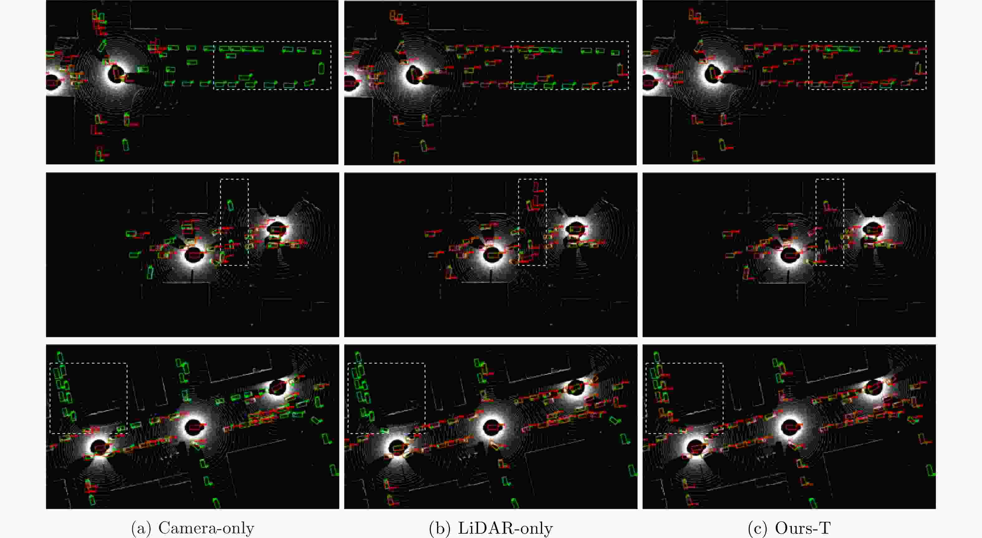
算法	Default		Culver city
算法	AP@0.5	AP@0.7	AP@0.5	AP@0.7
Camera-only	43.9	28.1	19.0	8.6
LiDAR-only	90.9	82.9	85.9	75.4
Hybrid-C	70.7	58.1	58.9	44.5
Hybrid-L	87.8	78.6	76.6	63.6

下载: 导出CSV

参考文献(30)

[1]	LIU Si, GAO Chen, CHEN Yuan, et al. Towards vehicle-to-everything autonomous driving: A survey on collaborative perception[EB/OL]. https://arxiv:abs/2308.16714, 2023.
[2]	HAN Yushan, ZHANG Hui, LI Huifang, et al. Collaborative perception in autonomous driving: Methods, datasets, and challenges[J]. IEEE Intelligent Transportation Systems Magazine, 2023, 15(6): 131–151. doi: 10.1109/MITS.2023.3298534
[3]	REN Shunli, CHEN Siheng, and ZHANG Wenjun. Collaborative perception for autonomous driving: Current status and future trend[C]. 2021 5th Chinese Conference on Swarm Intelligence and Cooperative Control, Singapore, Singapore, 2023: 682–692.
[4]	上官伟, 李鑫, 柴琳果, 等. 车路协同环境下混合交通群体智能仿真与测试研究综述[J]. 交通运输工程学报, 2022, 22(3): 19–40. doi: 10.19818/j.cnki.1671-1637.2022.03.002 SHANGGUAN Wei, LI Xin, CHAI Linguo, et al. Research review on simulation and test of mixed traffic swarm in vehicle-infrastructure cooperative environment[J]. Journal of Traffic and Transportation Engineering, 2022, 22(3): 19–40. doi: 10.19818/j.cnki.1671-1637.2022.03.002
[5]	CHEN Qi, TANG Sihai, YANG Qing, et al. Cooper: Cooperative perception for connected autonomous vehicles based on 3D point clouds[C]. 2019 IEEE 39th International Conference on Distributed Computing Systems (ICDCS), Dallas, USA, 2019: 514–524.
[6]	CHEN Qi, MA Xu, TANG Sihai, et al. F-cooper: Feature based cooperative perception for autonomous vehicle edge computing system using 3D point clouds[C]. 4th ACM/IEEE Symposium on Edge Computing, Arlington, USA, 2019: 88–100.
[7]	WANG T H, MANIVASAGAM S, LIANG Ming, et al. V2VNet: Vehicle-to-vehicle communication for joint perception and prediction[C]. 16th European Conference on Computer Vision, Glasgow, UK, 2020: 605–621.
[8]	XU Runsheng, XIANG Hao, XIA Xin, et al. OPV2V: An open benchmark dataset and fusion pipeline for perception with vehicle-to-vehicle communication[C]. 2022 International Conference on Robotics and Automation (ICRA), Philadelphia, USA, 2022: 2583–2589.
[9]	XU Runsheng, XIANG Hao, TU Zhengzhong, et al. V2x-ViT: Vehicle-to-everything cooperative perception with vision transformer[C]. 17th European Conference on Computer Vision, Tel Aviv, Israel, 2022: 107–124.
[10]	LI Yiming, REN Shunli, WU Pengxiang, et al. Learning distilled collaboration graph for multi-agent perception[C]. 34th International Conference on Neural Information Processing Systems, Virtual Online, 2021: 29541–29552.
[11]	LI Yiming, ZHANG Juexiao, MA Dekun, et al. Multi-robot scene completion: Towards task-agnostic collaborative perception[C]. 6th Conference on Robot Learning, Auckland, New Zealand, 2023: 2062–2072.
[12]	QIAO Donghao and ZULKERNINE F. Adaptive feature fusion for cooperative perception using LiDAR point clouds[C]. 2023 IEEE/CVF Winter Conference on Applications of Computer Vision, Waikoloa, USA, 2023: 1186–1195.
[13]	ZHANG Zijian, WANG Shuai, HONG Yuncong, et al. Distributed dynamic map fusion via federated learning for intelligent networked vehicles[C]. 2021 IEEE International Conference on Robotics and Automation (ICRA), Xi’an, China, 2021: 953–959.
[14]	WANG Binglu, ZHANG Lei, WANG Zhaozhong, et al. CORE: Cooperative reconstruction for multi-agent perception[C]. IEEE/CVF International Conference on Computer Vision, Paris, France, 2023: 8710–8720.
[15]	XU Runsheng, TU Zhengzhong, XIANG Hao, et al. CoBEVT: Cooperative bird’s eye view semantic segmentation with sparse transformers[C]. 6th Conference on Robot Learning, Auckland, New Zealand, 2022: 989–1000.
[16]	HU Yue, LU Yifan, XU Runsheng, et al. Collaboration helps camera overtake LiDAR in 3D detection[C]. 2023 IEEE/CVF Conference on Computer Vision and Pattern Recognition, Vancouver, Canada, 2023: 9243–9252.
[17]	党相卫, 秦斐, 卜祥玺, 等. 一种面向智能驾驶的毫米波雷达与激光雷达融合的鲁棒感知算法[J]. 雷达学报, 2021, 10(4): 622–631. doi: 10.12000/JR21036 DANG Xiangwei, QIN Fei, BU Xiangxi, et al. A robust perception algorithm based on a radar and LiDAR for intelligent driving[J]. Journal of Radars, 2021, 10(4): 622–631. doi: 10.12000/JR21036
[18]	CHEN Xiaozhi, MA Huimin, WAN Ji, et al. Multi-view 3D object detection network for autonomous driving[C]. 2017 IEEE Conference on Computer Vision and Pattern Recognition, Honolulu, USA, 2017: 6526–6534.
[19]	VORA S, LANG A H, HELOU B, et al. PointPainting: Sequential fusion for 3d object detection[C]. 2020 IEEE/CVF Conference on Computer Vision and Pattern Recognition, Seattle, USA, 2020: 4603–4611.
[20]	LIANG Tingting, XIE Hongwei, YU Kaicheng, et al. BEVFusion: A simple and robust LiDAR-camera fusion framework[C]. 36th International Conference on Neural Information Processing Systems, New Orleans, USA, 2022: 10421–10434.
[21]	LIU Zhijian, TANG Haotian, AMINI A, et al. BEVFusion: Multi-task multi-sensor fusion with unified bird’s-eye view representation[C]. 2023 IEEE International Conference on Robotics and Automation (ICRA), London, UK, 2023: 2774–2781.
[22]	JIAO Yang, JIE Zequn, CHEN Shaoxiang, et al. MSMDFusion: Fusing LiDAR and camera at multiple scales with multi-depth seeds for 3D object detection[C]. 2023 IEEE/CVF Conference on Computer Vision and Pattern Recognition, Vancouver, Canada, 2023: 21643–21652.
[23]	PRAKASH A, CHITTA K, and GEIGER A. Multi-modal fusion transformer for end-to-end autonomous driving[C]. 2021 IEEE/CVF Conference on Computer Vision and Pattern Recognition, Nashville, USA, 2021: 7073–7083.
[24]	XIANG Hao, XU Runsheng, and MA Jiaqi. HM-ViT: Hetero-modal vehicle-to-vehicle cooperative perception with vision transformer[EB/OL]. https://arxiv: abs/2304.10628, 2023.
[25]	READING C, HARAKEH A, CHAE J, et al. Categorical depth distribution network for monocular 3D object detection[C]. 2021 IEEE/CVF Conference on Computer Vision and Pattern Recognition, Nashville, USA, 2021: 8551–8560.
[26]	LANG A H, VORA S, CAESAR H, et al. PointPillars: Fast encoders for object detection from point clouds[C]. 2019 IEEE/CVF Conference on Computer Vision and Pattern Recognition, Long Beach, USA, 2019: 12689–12697.
[27]	VASWANI A, SHAZEER N, PARMAR N, et al. Attention is all you need[C]. 31st International Conference on Neural Information Processing Systems, Long Beach, USA, 2017: 6000–6010.
[28]	郭帅, 陈婷, 王鹏辉, 等. 基于角度引导Transformer融合网络的多站协同目标识别方法[J]. 雷达学报, 2023, 12(3): 516–528. doi: 10.12000/JR23014 GUO Shuai, CHEN Ting, WANG Penghui, et al. Multistation cooperative radar target recognition based on an angle-guided transformer fusion network[J]. Journal of Radars, 2023, 12(3): 516–528. doi: 10.12000/JR23014
[29]	XU Runsheng, GUO Yi, HAN Xu, et al. OpenCDA: An open cooperative driving automation framework integrated with co-simulation[C]. 2021 IEEE International Intelligent Transportation Systems Conference (ITSC), Indianapolis, USA, 2021: 1155–1162.
[30]	DOSOVITSKIY A, ROS G, CODEVILLA F, et al. CARLA: An open urban driving simulator[C]. 1st Annual Conference on robot learning, Mountain View, USA, 2017: 1–16.

施引文献

期刊类型引用(4)

1.	葛津津，周浩，凌天庆. 一种应用于脉冲探地雷达前端的探测子系统. 电子测量技术. 2022(04): 27-32 . 百度学术
2.	尹诗，郭伟. 用于探地雷达的超宽带天线设计与仿真. 电子设计工程. 2018(03): 98-102 . 百度学术
3.	宋立伟，张超，洪涛. 冲击波载荷对平面阵列天线电性能的影响. 电子机械工程. 2017(04): 1-5+58 . 百度学术
4.	尹德，叶盛波，刘晋伟，纪奕才，刘小军，方广有. 一种用于高速公路探地雷达的新型时域超宽带TEM喇叭天线. 雷达学报. 2017(06): 611-618 . 本站查看

其他类型引用(6)

资源附件(0)

访问统计

图(4) / 表(2)

计量

文章访问数: 2911
HTML全文浏览量: 289
PDF下载量: 621
被引次数: 10

1. Introduction
2. Conformal FDA-MIMO Radar
2.1 General conformal FDA-MIMO signal model
2.2 CRLB of conformal FDA-MIMO
3. Reduced-Dimension Target Parameter Estimation Algorithm
4. Simulation Results
4.1 Analysis of computational complexity
4.2 Single target parameter estimation
4.3 Multiple targets parameter estimation
5. Conclusion

1. Introduction
2. Conformal FDA-MIMO Radar
2.1 General conformal FDA-MIMO signal model
2.2 CRLB of conformal FDA-MIMO
3. Reduced-Dimension Target Parameter Estimation Algorithm
4. Simulation Results
4.1 Analysis of computational complexity
4.2 Single target parameter estimation
4.3 Multiple targets parameter estimation
5. Conclusion

参考文献(30)

施引文献

资源附件(0)

访问统计

基于多传感器融合的协同感知方法

DOI: 10.12000/JR23184

通讯作者:
周天飞 ztfei.debug@gmail.com

计量

Collaborative Perception Method Based on Multisensor Fusion

Corresponding author: ZHOU Tianfei, ztfei.debug@gmail.com

1. Introduction

2. Conformal FDA-MIMO Radar

2.1 General conformal FDA-MIMO signal model

2.2 CRLB of conformal FDA-MIMO

3. Reduced-Dimension Target Parameter Estimation Algorithm

4. Simulation Results

4.1 Analysis of computational complexity

4.2 Single target parameter estimation

4.3 Multiple targets parameter estimation

5. Conclusion

期刊类型引用(4)

其他类型引用(6)

计量

目录

1. Introduction

2. Conformal FDA-MIMO Radar

2.1 General conformal FDA-MIMO signal model

2.2 CRLB of conformal FDA-MIMO

3. Reduced-Dimension Target Parameter Estimation Algorithm

4. Simulation Results

4.1 Analysis of computational complexity

4.2 Single target parameter estimation

4.3 Multiple targets parameter estimation

5. Conclusion

期刊介绍

联系我们

基于多传感器融合的协同感知方法

DOI: 10.12000/JR23184

通讯作者: 周天飞 ztfei.debug@gmail.com

计量

出版历程

Collaborative Perception Method Based on Multisensor Fusion

Corresponding author: ZHOU Tianfei, ztfei.debug@gmail.com

1. Introduction

2. Conformal FDA-MIMO Radar

2.1 General conformal FDA-MIMO signal model

2.2 CRLB of conformal FDA-MIMO

3. Reduced-Dimension Target Parameter Estimation Algorithm

4. Simulation Results

4.1 Analysis of computational complexity

4.2 Single target parameter estimation

4.3 Multiple targets parameter estimation

5. Conclusion

期刊类型引用(4)

其他类型引用(6)

计量

出版历程

目录

1. Introduction

2. Conformal FDA-MIMO Radar

2.1 General conformal FDA-MIMO signal model

2.2 CRLB of conformal FDA-MIMO

3. Reduced-Dimension Target Parameter Estimation Algorithm

4. Simulation Results

4.1 Analysis of computational complexity

4.2 Single target parameter estimation

4.3 Multiple targets parameter estimation

5. Conclusion

期刊介绍

联系我们

通讯作者:
周天飞 ztfei.debug@gmail.com