Loading [MathJax]/jax/element/mml/optable/BasicLatin.js

基于INet的雷达图像杂波抑制和目标检测方法

牟效乾 陈小龙 关键 周伟 刘宁波 董云龙

陈慧, 田湘, 李子豪, 等. 共形FDA-MIMO雷达降维目标参数估计研究[J]. 雷达学报, 2021, 10(6): 811–821. DOI: 10.12000/JR21197
引用本文: 牟效乾, 陈小龙, 关键, 等. 基于INet的雷达图像杂波抑制和目标检测方法[J]. 雷达学报, 2020, 9(4): 640–653. doi: 10.12000/JR20090
CHEN Hui, TIAN Xiang, LI Zihao, et al. Reduced-dimension target parameter estimation for conformal FDA-MIMO radar[J]. Journal of Radars, 2021, 10(6): 811–821. DOI: 10.12000/JR21197
Citation: MOU Xiaoqian, CHEN Xiaolong, GUAN Jian, et al. Clutter suppression and marine target detection for radar images based on INet[J]. Journal of Radars, 2020, 9(4): 640–653. doi: 10.12000/JR20090

基于INet的雷达图像杂波抑制和目标检测方法

DOI: 10.12000/JR20090
基金项目: 国家自然科学基金(U1933135, 61931021),山东省重点研发计划(2019GSF111004, 2019JZZY010415),基础加强计划技术领域基金(2102024)
详细信息
    作者简介:

    牟效乾(1995–),男,山东烟台人,硕士生。研究领域包括智能雷达信号处理、动目标检测等。E-mail: 1012226010@qq.com

    陈小龙(1985–),男,山东烟台人,博士,副教授。研究领域包括雷达信号处理、海杂波抑制、雷达智能探测等。入选中国科协“青年人才托举工程”,被评为中国电子学会优秀科技工作者,获中国电子学会优博,中国专利优秀奖,军队科技进步一等奖等。E-mail: cxlcxl1209@163.com

    关 键(1968–),男,辽宁锦州人,教授,博士生导师。主要研究方向包括雷达目标检测与跟踪、侦察图像处理和信息融合。获国家科技进步二等奖1项、军队科技进步一等奖2项,山东省技术发明一等奖1项;“百千万人才工程”国家级人选,入选教育部新世纪优秀人才支持计划。E-mail: guanjian_68@163.com

    周 伟(1980–),男,湖北黄石人,副教授,主要研究方向为多源信息融合、侦察图像处理、目标检测与识别。E-mail: yeaweam@gmail.com

    刘宁波(1983–),男,海军航空大学信息融合研究所副教授、博士,主要研究方向为雷达信号智能处理、海上目标探测技术。E-mail: lnb198300@163.com

    董云龙(1974–),男,天津宝坻人,教授,主要研究方向为多传感器信息融合。E-mail: china_dyl@sina.com

    通讯作者:

    陈小龙 cxlcxl1209@163.com

  • 责任主编:许述文 Corresponding Editor: XU Shuwen
  • 中图分类号: TN957.51

Clutter Suppression and Marine Target Detection for Radar Images Based on INet

Funds: The National Natural Science Foundation of China (U1933135, 61931021), The Key Research and Development Program of Shandong Province (2019GSF111004, 2019JZZY010415), The Fundamental Strengthening Technology Program (2102024))
More Information
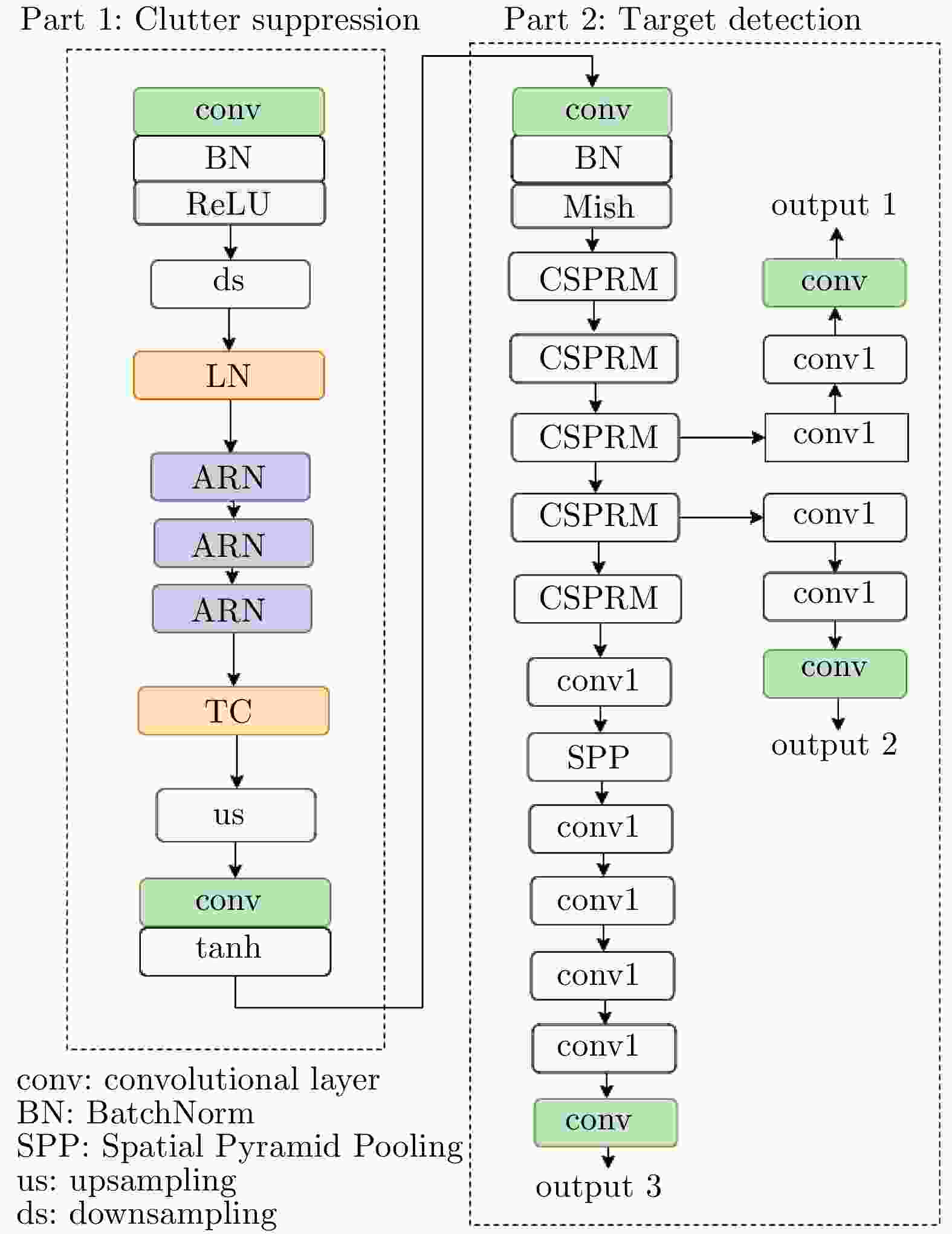
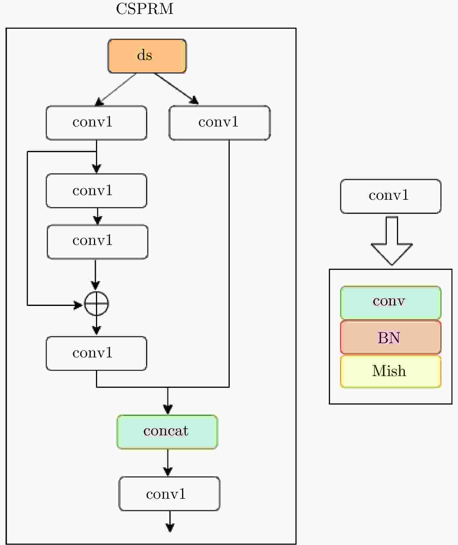
  • 摘要: 强海杂波与海面目标的复杂特性使得海面目标回波微弱,有效的海杂波抑制和稳健快速的目标检测是雷达对海上目标探测需考虑的重要因素。然而,现有的海面目标检测算法对于复杂环境下的目标检测性能有限,环境和目标特性适应性差。该文设计了一种杂波抑制和目标检测融合网络(INet),通过层归一化-传递和连接方法提取关键目标特征,采用注意力网络抑制杂波和增强目标,构建跨阶段局部残差网络保证检测网络的轻量化和准确性。基于导航雷达在多种观测条件下采集的回波数据,构建了海面目标雷达图像数据集;通过模型的预训练和平面位置显示器(PPI)图像的帧间积累对INet进行了优化,得到了Optimized INet(O-INet)模型。经过多种天气条件下实测数据测试和验证,并与YOLOv3, YOLOv4,双参数CFAR和二维CA-CFAR对比后证明,所提方法在提高检测概率、降低虚警率和复杂条件下的强泛化能力有显著优势。


  • In recent years, Frequency Diverse Array (FDA) radar has received much attention due to its range-angle-time-dependent beampattern[1,2]. Combining the advantages of FDA and traditional phased array Multiple-Input Multiple-Output (MIMO) radar in the degree of freedom, the FDA Multiple-Input Multiple Output (FDA-MIMO) radar was proposed in Ref. [3] and applied in many fields[4-9]. For parameter estimation algorithm, the authors first proposed a FDA-MIMO target localization algorithm based on sparse reconstruction theory[10], and an unbiased joint range and angle estimation method was proposed in Ref. [11]. The work of Ref. [12] further proved that the FDA-MIMO is superior to traditional MIMO radar in range and angle estimation performance, and the authors of Ref. [13] introduced a super-resolution MUSIC algorithm for target location, and analyzed its resolution threshold. Meanwhile, high-resolution Doppler processing is utilized for moving target parameter estimation[14]. The Estimation of Signal Parameters via Rotational Invariance Technique (ESPRIT) and PARAllel FACtor (PARAFAC) was proposed in Ref. [15], which is a search-free algorithm for FDA-MIMO.

    Moreover, the research of conformal array has received more and more attention. Conformal array is a non-planar array that can be completely attached to the surface of the carrier[16]. It has significant advantages such as reducing the aerodynamic impact on the carrier and smaller radar cross section[17]. In addition, conformal array can achieve wide-angle scanning with a lower SideLobe Level (SLL)[18]. Different from traditional arrays, the element beampattern of conformal array needs to be modeled separately in the parameter estimation due to the difference of carrier curvature[19-21].

    As far as we know, most of the existing researches on FDA-MIMO are based on linear array, while there is little research on the combination of FDA-MIMO and conformal array[22]. In this paper, we replace the receiving array in the traditional FDA-MIMO with conformal array. Compared with conventional FDA-MIMO, conformal FDA-MIMO inherits the merits of conformal array and FDA-MIMO, which can effectively improve the stealth and anti-stealth performance of the carrier, and reduce the volume and the air resistance of the carrier. For conformal FDA-MIMO, we further study the parameters estimation algorithm. The major contributions of this paper are summarized as follows:

    (1) A conformal FDA-MIMO radar model is first formulated.

    (2) The parameter estimation Cramér-Rao Lower Bound (CRLB) for conformal FDA-MIMO radar is derived.

    (3) Inspired by the existing work of Refs. [23,24], a Reduced-Dimension MUSIC (RD-MUSIC) algorithm for conformal FDA-MIMO radar is correspondingly proposed to reduce the complexity.

    The rest of the paper consists of four parts. Section 2 formulates the conformal FDA-MIMO radar model, and Section 3 derives a RD-MUSIC algorithm for conformal FDA-MIMO radar. Simulation results for conformal FDA-MIMO radar with semi conical conformal receiving array are provided in Section 4. Finally, conclusions are drawn in Section 5.

    For the convenience of analysis, we consider a monostatic conformal FDA-MIMO radar which is composed by a M-element linear FDA transmitting array and a N-element conformal receiving array, as shown in Fig. 1. d denotes the inter-element spacing, the carrier frequency at the mth transmitting element is fm=f1+Δf(m1), m=1,2,,M where f1 is the transmission frequency of the first antenna element, which is called as reference frequency, and Δf is the frequency offset between the adjacent array elements.

    Figure  1.  Conformal FDA-MIMO radar

    The complex envelope of the transmitted signal of the mth transmitting element is denoted as φm(t), assume the transmitting waveforms have orthogonality,

    Tpφm(t)φm1(tτ)dt=0,m1m (1)

    where τ denotes the time delay, Tp denotes the pulse duration, and () is conjugate operator. The signal transmitted from the mth element can be expressed as

    sm(t)=am(t,θ,ϕ,r)φm(t),0tTp (2)

    where

    am(t,θ,ϕ,r)=exp{j2π((m1)Δfrcf1(m1)dsinαc(m1)Δft)} (3)

    is the mth element of the transmitting steering vector according to the phase difference between adjacent elements, the angle between far-field target and transmitting array is denoted as α=arcsin(sinθcosϕ), where arcsin() denotes arcsine operator, α can be calculated by using the inner product between the target vector and unit vector along the X-axis. θ,ϕ,r are the elevation, azimuth and range between the target and the origin point, respectively. The phase difference between adjacent elements is

    Δψt0=2π(Δfrcf1dsinαcΔft) (4)

    where c is light speed. For far-field target P(r,θ,ϕ), the transmitting steering vector is

    a0(t,θ,ϕ,r)=[1,exp{jΔψt0},,exp{j(M1)Δψt0}]T (5)

    For the conformal receiving array, as shown in Fig. 1(b), the time delay between target P(r,θ,ϕ) and the nth receiving array element is

    τn=rn/c (6)

    where rn is the range between target and the nth receiving array element. For far-field assumption, the rn can be approximated as

    rnrpnr (7)

    where r denotes the range between the target and the origin point, pn=xnex+yney+znez denotes the position vector from the nth element to origin point, and r=sinθcosϕex+sinθsinϕey+cosθez is the unit vector in target orientation, where ex,ey and ez are the unit vectors along the X- , Y- , and Z-axis, respectively. (xn,yn,zn) are the coordinates of the nth element in the Cartesian coordinate system. For simplicity, we let u=sinθcosϕ, v=sinθcosϕ, so the time delay τn=(r(uxn+vyn+cosθzn))/c. The time delay between the first element and the nth element at the receiving array is expressed as

    Δτrn=τ1τn=u(xnx1)+v(yny1)+cosθ(znz1)c (8)

    And the corresponding phase difference between the first element and the nth element is

    ΔψRn=2πf1Δτrn (9)

    Consequently, the receiving steering vector is

    b(θ,ϕ)=[r1(θ,ϕ),r2(θ,ϕ)exp(jΔψr2),,rN(θ,ϕ)exp(jΔψrN)]T (10)

    where rn(θ,ϕ) is the nth conformal receiving array element beampattern which should be designed in its own local Cartesian coordinate system. In this paper, we utilize Euler rotation method to establish transformation frame between local coordinate system and global coordinate system[25,26].

    Then the total phase difference between adjacent transmitting array elements can be rewritten as

    Δψt=2π(Δf2rcf1dsinαcΔft) (11)

    where the factor 2r in the first term represents the two-way transmission and reception, and the correspondingly transmitting steering vector is written as

    a(t,θ,ϕ,r)=[1,exp{jΔψt},,exp{j(M1)Δψt}]T (12)

    Assuming L far-field targets are located at (θi,ϕi,Ri), i=1,2,,L and snapshot number is K. After matched filtering, the received signal can be formulated as following matrix (13,14)

    X=AS+N (13)

    where the array manifold A is expressed as

    A=[at,r(θ1,ϕ1,r1),,at,r(θL,ϕL,rL)]=[b(θ1,ϕ1)a(θ1,ϕ1,r1),,b(θL,ϕL)a(θL,ϕL,rL)] (14)

    where at,r(θ,ϕ,r) is the joint transmitting-receiving steering vector, S=[s(t1),s(t2),,s(tK)]CL×K and NCMN×K denote the signal matrix and noise matrix, respectively, where noise follows the independent identical distribution, and denotes Kronecker product.

    a(θ,ϕ,r)=[1exp{j2π(2Δfrcf1dsinαc)}exp{j2π(M1)(2Δfrcf1dsinαc)}] (15)

    which can be expressed as

    a(θ,ϕ,r)=a(θ,ϕ)a(r) (16)

    where

    a(r)=[1,exp(j2π2Δfrc),,exp(j2π(M1)2Δfrc)]T (17)
    a(θ,ϕ)=[1,exp(j2πf1dsinαc),,exp[j2π(M1)f1dsinαc]]T (18)

    and represents Hadamard product operator.

    The CRLB can be obtained from the inverse of Fisher information matrix[27,28], which establishes a lower bound for the variance of any unbiased estimator. We employ the CRLB for conformal FDA-MIMO parameter estimation to evaluate the performance of some parameter estimation algorithms.

    The discrete signal model is

    x[k]=at,r(θ,ϕ,r)s[k]+N[k],k=1,2,,K (19)

    For the sake of simplification, we take at,r as the abbreviation of at,r(θ,ϕ,r).

    The Probability Distribution Function (PDF) of the signal model with K snapshots is

    p(x|θ,ϕ,r)=1(2πσ2n)K2exp(1σ2n(xat,rs)H(xat,rs)) (20)

    where x=[x(1),x(2),,x(K)] and s=[s(1),s(2),,s(K)].

    The CRLB matrix form of elevation angle, azimuth angle and range is given by Eq. (21), diagonal elements {Cθθ,Cϕϕ,Crr} represent CRLB of estimating elevation angle, azimuth angle and range, respectively.

    CRLB=[CθθCθϕCθrCϕθCϕϕCϕrCrθCrϕCrr]=FIM1=[F11F12F13F21F22F23F31F32F33] (21)

    The elements of Fisher matrix can be expressed as

    Fij=E[2ln(p(xθ,ϕ,r))xixj],i,j=1,2,3 (22)

    In the case of K snapshots, PDF can be rewritten as

    p(x|θ,ϕ,r)=Cexp{1σ2nKn=1(x[k]at,rs[k])H(x[k]at,rs[k])} (23)

    where C is a constant, natural logarithm of Eq. (23) is

    ln(p(x|θ,ϕ,r))=ln(C)1σ2nKk=1(x[k]at,rs[k])H(x[k]at,rs[k]) (24)

    where ln() represents the logarithm operator. The first entry of Fisher matrix can be expressed as

    F11=E[2ln(p(x|θ,ϕ,r))θ2] (25)

    Correspondingly, the first derivative of natural logarithm is given by

    ln(p(x|θ,ϕ,r))θ=1σ2nKk=1(xH[k]at,rθs[k]aHt,rθs[k]x[k]+aHt,rθat,rs2[n]a+aHt,rat,rθs2[n]) (26)

    Then we can obtain the second derivative of

    2ln(p(x|θ,ϕ,r))θ2=1σ2nKk=1(x[k]H2at,rθ2s[k]2aHt,rθ2s(k)x[k]+2aHt,rθ2at,rs[k]2+aHt,rθat,rθs[k]2+aHt,rθat,rθs[k]2+aHt,r2at,rθ2s[k]2) (27)

    And then we have

    Kk=1x[k]=Kk=1at,rs[k]+N[k]=at,r(θ,ϕ,r)Kk=1s[k] (28)

    and

    Kk=1s2[k]=Kvar(s[k])=Kσ2s (29)

    where var() is a symbol of variance. Therefore, the PDF after quadratic derivation can be written as

    E[2ln(p(x|θ,ϕ,r))θ2]=Kσ2sσ2n(aHt,rθat,rθ+aHt,rθat,rθ)=2Kσ2sσ2nat,rθ2 (30)

    where denotes 2-norm. Similarly, the other elements of the Fisher matrix can also be derived in the similar way, so the Fisher matrix can be expressed as

    CRLB1=FIM=2Kσ2sσ2n[aθ2FIM12FIM13FIM21aϕ2FIM23FIM31FIM32ar2] (31)

    where

    FIM12=12[aHt,rθat,rϕ+aHt,rϕat,rθ],
    FIM13=12[aHt,rθat,rr+aHt,rrat,rθ],
    FIM21=12[aHt,rϕat,rθ+aHt,rθat,rϕ],
    FIM23=12[aHt,rϕat,rr+aHt,rrat,rϕ],
    FIM31=12[aHt,rrat,rθ+aHt,rθat,rr],
    FIM32=12[aHt,rrat,rϕ+aHt,rϕat,rr],
    σ2sσ2n=SNR

    Finally, the CRLB of conformal FDA-MIMO can be calculated by the inverse of Fisher matrix.

    The covariance matrix of the conformal FDA-MIMO receiving signal can be written as

    RX=ARsAH+σ2IMN (32)

    where Rs represents the covariance matrix of transmitting signal, IMN denotes MN dimensional identity matrix. For independent target signal and noise, RX can be decomposed as

    RX=USΛSUHS+UnΛnUHn (33)

    The traditional MUSIC algorithm is utilized to estimate the three-dimensional parameters {θ,ϕ,r}, MUSIC spectrum can be expressed as

    PMUSIC(θ,ϕ,r)=1aHt,r(θ,ϕ,r)UnUHnat,r(θ,ϕ,r) (34)

    The target location can be obtained by mapping the peak indexes of MUSIC spectrum.

    Traditional MUSIC parameter estimation algorithm is realized by 3D parameter search, which has good performance at the cost of high computational complexity. When the angular scan interval is less than 0.1°, the running time of single Monte-Carlo simulation is in hours, which is unpracticable for us to analysis conformal FDA-MIMO estimation performance by hundreds of simulations.

    In order to reduce the computation complexity of the parameter estimation algorithm for conformal FDA-MIMO, we propose a RD-MUSIC algorithm, which has a significant increase in computing speed at the cost of little estimation performance loss.

    At first, we define

    V(θ,ϕ,r)=aHt,r(θ,ϕ,r)HUnUHnat,r(θ,ϕ,r)=[b(θ,ϕ)a(θ,ϕ,r)]HUnUHn[b(θ,ϕ)a(θ,ϕ,r)] (35)

    Eq. (35) can be further calculated by

    V(θ,ϕ,r)=aH(θ,ϕ,r)[b(θ,ϕ)IM]H×UnUHn[b(θ,ϕ)IM]a(θ,ϕ,r)=aH(θ,ϕ,r)Q(θ,ϕ)a(θ,ϕ,r) (36)

    where Q(θ,ϕ)=[b(θ,ϕ)IM]HUnUHn[b(θ,ϕ)IM],

    Eq. (36) can be transformed into a quadratic programming problem. To avoid a(θ,ϕ,r)=0M, we add a constraint eH1a(θ,ϕ,r)=1, where e1 denotes unit vector. As a result, the quadratic programming problem can be redefined as

    {min (37)

    The penalty function can be constructed as

    \begin{split} L(\theta ,\phi ,r) =& {{\boldsymbol{a}}^{\rm{H}}}(\theta ,\phi ,r){\boldsymbol{Q}}(\theta ,\phi ){\boldsymbol{a}}(\theta ,\phi ,r) \\ & - \mu \left({\boldsymbol{e}}_1^{\text{H}}{\boldsymbol{a}}(\theta ,\phi ,r) - 1\right) \\ \end{split} (38)

    where \mu is a constant, because {\boldsymbol{a}}\left( {\theta ,\phi ,r} \right) = {\boldsymbol{a}}\left( {\theta ,\phi } \right) \odot {\boldsymbol{a}}\left( r \right), so we can obtain

    \begin{split} \frac{{\partial L(\theta ,\phi ,r)}}{{\partial {\boldsymbol{a}}(r)}} =& 2{\rm{diag}}\left\{ {{\boldsymbol{a}}(\theta ,\phi )} \right\}{\boldsymbol{Q}}(\theta ,\phi ){\boldsymbol{a}}(\theta ,\phi ,r) \\ & - \mu {\rm{diag}}\left\{ {{\boldsymbol{a}}(\theta ,\phi )} \right\}{\boldsymbol{e}}_{\boldsymbol{1}}^{} \end{split} (39)

    where {\rm{diag}}( \cdot ) denotes diagonalization.

    And then let \dfrac{{\partial L(\theta ,\phi ,r)}}{{\partial {\boldsymbol{a}}(r)}} = 0, we can get

    {\boldsymbol{a}}\left( r \right) = \varsigma {{\boldsymbol{Q}}^{ - 1}}(\theta ,\phi ){\boldsymbol{e}}_1^{}./{\boldsymbol{a}}(\theta ,\phi ) (40)

    where \varsigma is a constant, ./ denotes the division of the corresponding elements, which is opposite of Hadamard product. Substituting the constraint {\boldsymbol{e}}_1^{\rm{H}}{\boldsymbol{a}}(\theta ,\phi ,r) = 1 into {\boldsymbol{a}}\left( r \right) , we can obtain \varsigma = 1/({\boldsymbol{e}}_1^{\rm{H}}{{\boldsymbol{Q}}^{ - 1}} \cdot(\theta ,\phi ){\boldsymbol{e}}_1 ), then {\boldsymbol{a}}\left( r \right) can be expressed as

    {\boldsymbol{a}}\left( r \right) = \frac{{{{\boldsymbol{Q}}^{ - 1}}\left( {\theta ,\phi } \right){{\boldsymbol{e}}_1}}}{{{\boldsymbol{e}}_1^{\rm{H}}{{\boldsymbol{Q}}^{ - 1}}\left( {\theta ,\phi } \right){{\boldsymbol{e}}_1}}}./{\boldsymbol{a}}\left( {\theta ,\phi } \right) (41)

    Substituting {\boldsymbol{a}}\left( r \right) into Eq. (37), the target azimuths and elevations can be estimated by searching two-dimensional azimuth-elevation spectrum,

    \begin{split} \hfill \lt \hat \theta ,\hat \phi \gt =& {\text{arg}}\mathop {\min }\limits_{\theta ,\phi } \frac{1}{{{\boldsymbol{e}}_1^{\text{H}}{{\boldsymbol{Q}}^{ - 1}}(\theta ,\phi ){{\boldsymbol{e}}_{\boldsymbol{1}}}}} \\ =& {\text{arg}}\mathop {\max }\limits_{\theta ,\phi } {\boldsymbol{e}}_1^{\text{H}}{{\boldsymbol{Q}}^{ - 1}}(\theta ,\phi ){{\boldsymbol{e}}_{\boldsymbol{1}}} \end{split} (42)

    Given azimuth-elevation estimations obtained by mapping the L peak points, the range information can be obtained by searching range-dimensional spectrum,

    P\left({\hat \theta _i},{\hat \phi _i},r\right){\text{ }} = \frac{1}{{{\boldsymbol{a}}_{t,r}^{\rm{H}}\left({{\hat \theta }_i},{{\hat \phi }_i},r\right){{\boldsymbol{U}}_n}{\boldsymbol{U}}_n^{\rm{H}}{{\boldsymbol{a}}_{t,r}}\left({{\hat \theta }_i},{{\hat \phi }_i},r\right)}} (43)

    For conformal array, different array layouts produce different element patterns. We select the semi conical conformal array which is shown in Fig. 2 as the receiving array for the following simulation.

    Figure  2.  Conformal FDA-MIMO semi conical receiving array

    The simulation parameters are provided as follows: M = 10,N = 7,{f_1} = 10\;{\rm{GHz}},\Delta f = 3\;{\rm{kHz}}, d = \lambda /2 = c/2{f_1} and c = 3 \times {10^8}\;{\rm{m}}/{\rm{s}}.

    We first analyze the computational complexity of the algorithms in respect of the calculation of covariance matrix, the eigenvalue decomposition of the matrix and the spectral search. The main complexity of the MUISC algorithm and our proposed RD-MUISC algorithm are respectively as

    O\left(KL{({MN})^2} + 4/3{({MN})^{\text{3}}}{{ + L}}{\eta _1}{\eta _2}{\eta _3}{({MN})^2} \right) (44)
    O\left(KL{({MN})^2} + 4/3{({MN})^{\text{3}}}{{ + L}}{\eta _1}{\eta _2}{({MN})^2} + L{\eta _3}{({MN})^2}\right) (45)

    Where K and L denote snapshot number and signal sources number, {\eta _1},{\eta _2} and {\eta _3} represent search number in three-dimensional parameter \theta ,\phi ,r , respectively.

    From Eq. (44) and Eq. (45), we can see that the main complexity reduction of the RD-MUSIC algorithm lies in the calculation of the spectral search function. With the increase of the search accuracy, the complexity reduction is more significant.

    The computational complexity of algorithms is compared in Fig. 3. It can be seen from Fig. 3 that the difference of computational complexity between the two algorithms gradually increases with the increase of search accuracy. In the case of high accuracy, the computational efficiency of RD-MUSIC algorithm can reach more than {10^3} times of the traditional MUSIC algorithm. The simulation results show that RD-MUSIC algorithm has advantage in computing efficiency for conformal FDA-MIMO.

    Figure  3.  Comparison of computational complexity under different scan spacing

    In order to illustrate the effectiveness of the RD-MUSIC algorithm for a single target which is located at ({30^\circ },{20^\circ },10\;{\rm{km}}), we first give the parameter estimation probability of success with 1000 times Monte Carlo simulation, as shown in Fig. 4, the criterion of successful estimation is defined as the absolute difference between the estimation value and the actual value is less than a designed threshold \varGamma . More specifically, the criterion is \left| {\hat \theta - \theta } \right| < {\varGamma _\theta },\left| {\hat \phi - \phi } \right| < {\varGamma _\phi },\left| {\hat r - r} \right| < {\varGamma _r} , and suppose {\varGamma _\theta } = \varGamma \times {1^\circ },{\varGamma _\phi } = \varGamma \times {1^\circ },{\varGamma _r} = \varGamma \times 100\;{\rm{m}}, in the simulation, as well as the search paces are set as \left[ {{{0.05}^\circ },{{0.05}^\circ },0.05\;{\rm{km}}} \right], respectively. From Fig. 4, we can see that the probability of success gets higher as \varGamma gets bigger, which is consistent with expected.

    Figure  4.  The parameter estimation probability of RD-MUSIC algorithm with different thresholds

    Then, we consider the single target parameter estimation performance, Fig. 5 shows the RMSE of different algorithms with the increase of SNR under 200 snapshots condition, and Fig. 6 demonstrates the RMSE of different algorithms with the increase of snapshot number when SNR=0 dB. As shown in Fig. 5 and Fig. 6, the RMSEs of conformal FDA-MIMO gradually descend with the increasing of SNRs and snapshots, respectively. At the same time, the performance of traditional algorithm is slightly higher than RD-MUSIC algorithm. When the number of snapshots is more than 200, the difference of RMSEs is less than {10^{ - 1}} . Therefore, the performance loss of RD-MUSIC algorithm is acceptable compared with the improved computational speed. Note that, here we set 100 times Monte Carlo simulation to avoid running too long.

    Figure  5.  The RMSE versus snapshot for single target case
    Figure  6.  The RMSE versus SNR for two targets case

    Without loss of generality, we finally consider two targets which are located at ({30^\circ },{20^\circ }, 10\;{\rm{km}}) and ({30^\circ },{20^\circ },12\;{\rm{km}}), respectively, the remaining parameters are the same as single target case. Fig. 7 and Fig. 8 respectively show the RMSE of different algorithms with the increase of SNR and snapshot number in the case of two targets.

    Figure  7.  The RMSE versus snapshot for two targets case
    Figure  8.  The RMSE versus snapshot for two targets case

    It can be seen from Fig. 7 that the RMSE curve trend of angle estimation is consistent with that of single target case. The performance of traditional MUSIC algorithm is slightly better than that of RD-MUSIC algorithm. In the range dimension, the performance of traditional algorithm hardly changes with SNR, and RD-MUSIC algorithm is obviously better than traditional MUSIC algorithm. The proposed RD-MUSIC algorithm first estimates the angles, and then estimates the multiple peaks from range-dimensional spectrum, which avoids the ambiguity in the three-dimensional spectral search. Therefore, the RD-MUSIC algorithm has better range resolution for multiple targets estimation.

    In this paper, a conformal FDA-MIMO radar is first established, and the corresponding signal receiving mathematical model is formulated. In order to avoid the computational complexity caused by three-dimensional parameter search of MUSIC algorithm, we propose a RD-MUSIC algorithm by solving a quadratic programming problem. Simulation results show that the RD-MUSIC algorithm has comparative angle estimation performance with that of traditional MUSIC algorithm while greatly reducing the computation time. And the RD-MUSIC algorithm has better range estimation performance for multiple targets.

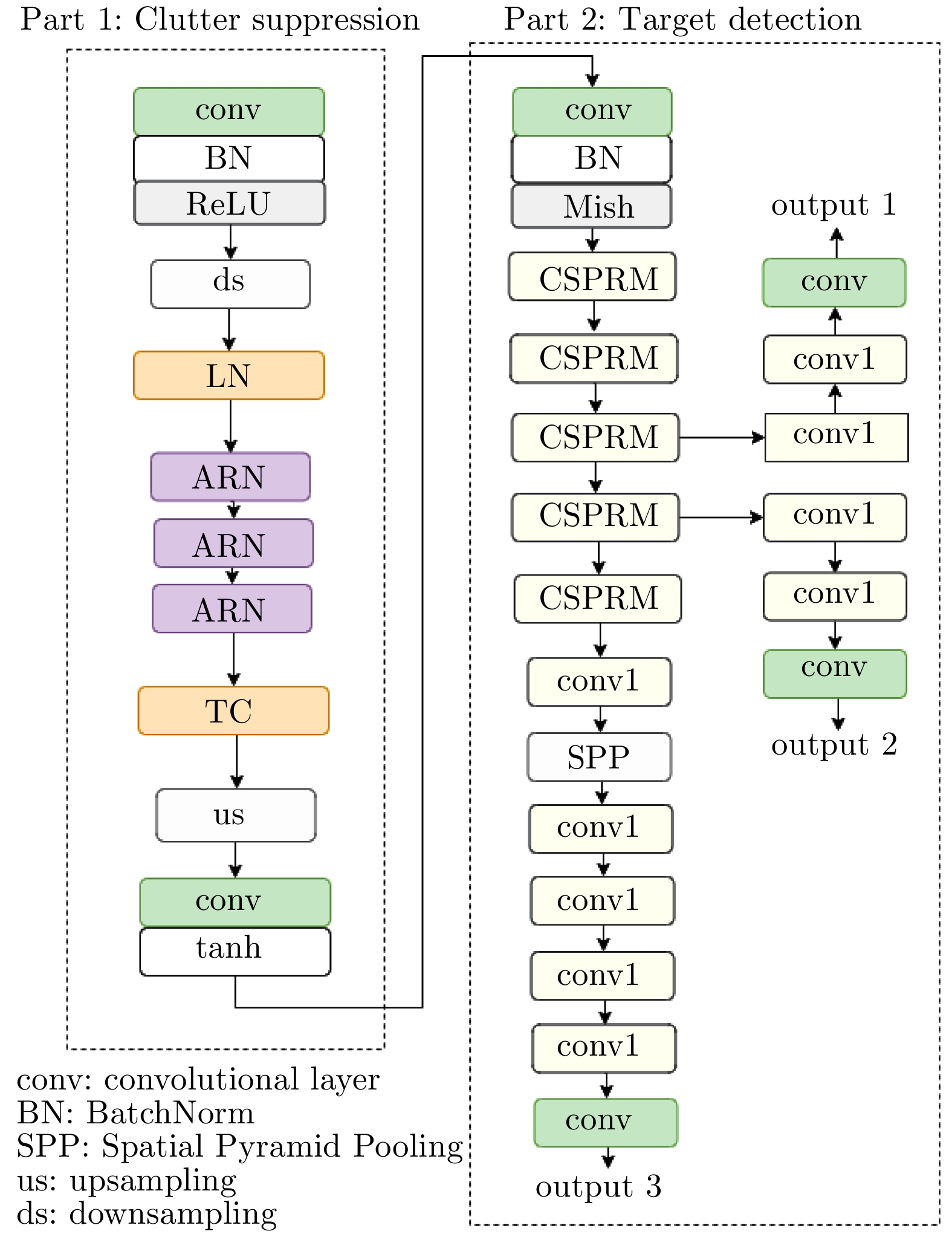
  • 图  1  INet网络结构

    Figure  1.  The network structure of INet

    图  2  ARN网络结构

    Figure  2.  The network structure of ARN

    图  3  CSPRM结构

    Figure  3.  The network structure of CSPRM

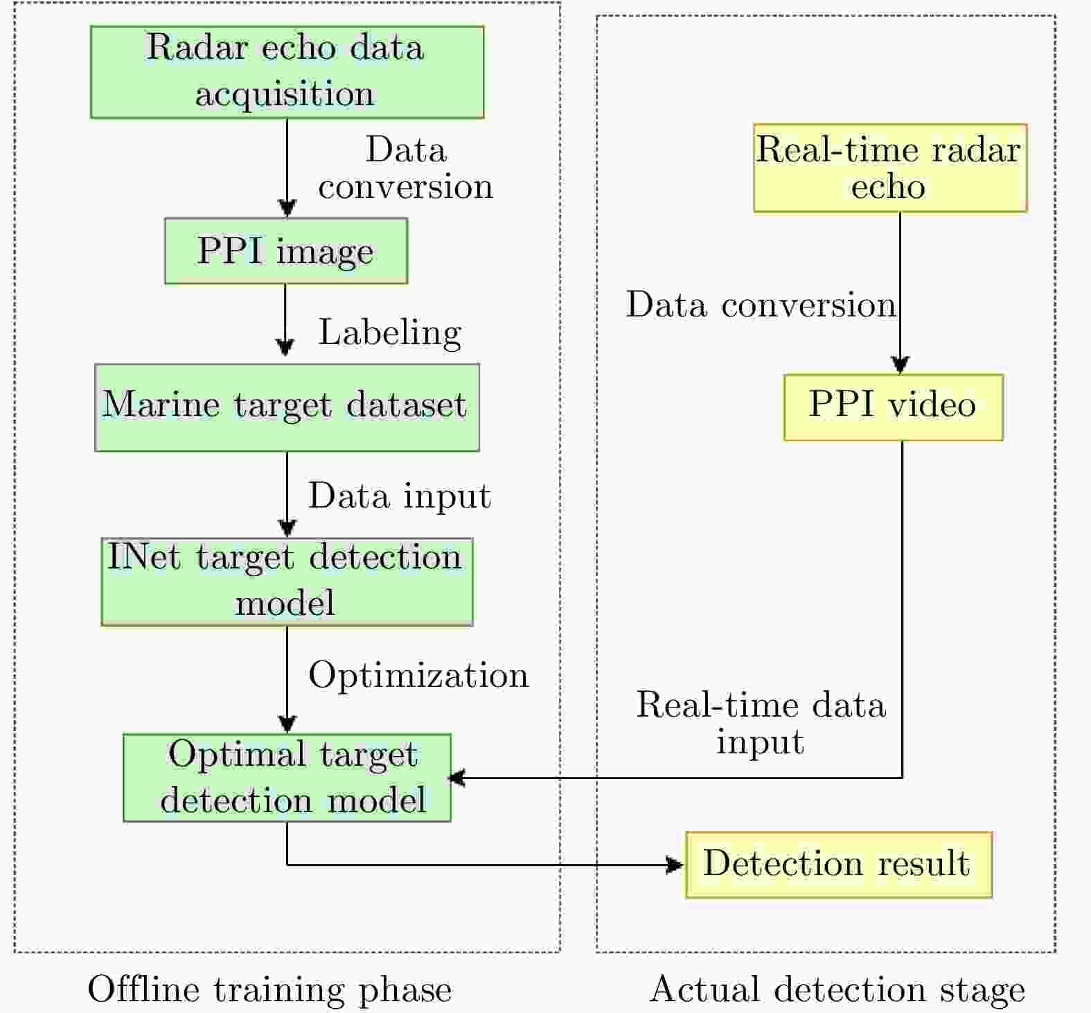
    图  4  基于INet的目标检测算法流程图

    Figure  4.  Flowchart of target detection algorithm based on INet

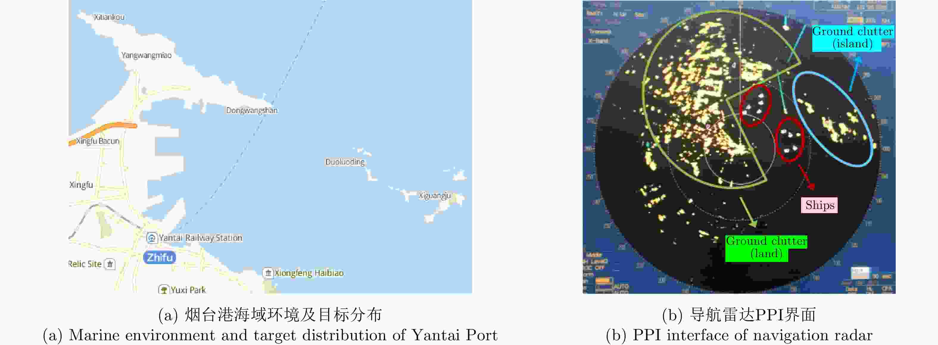
    图  5  探测环境及雷达PPI界面

    Figure  5.  Detection environment and radar PPI interface

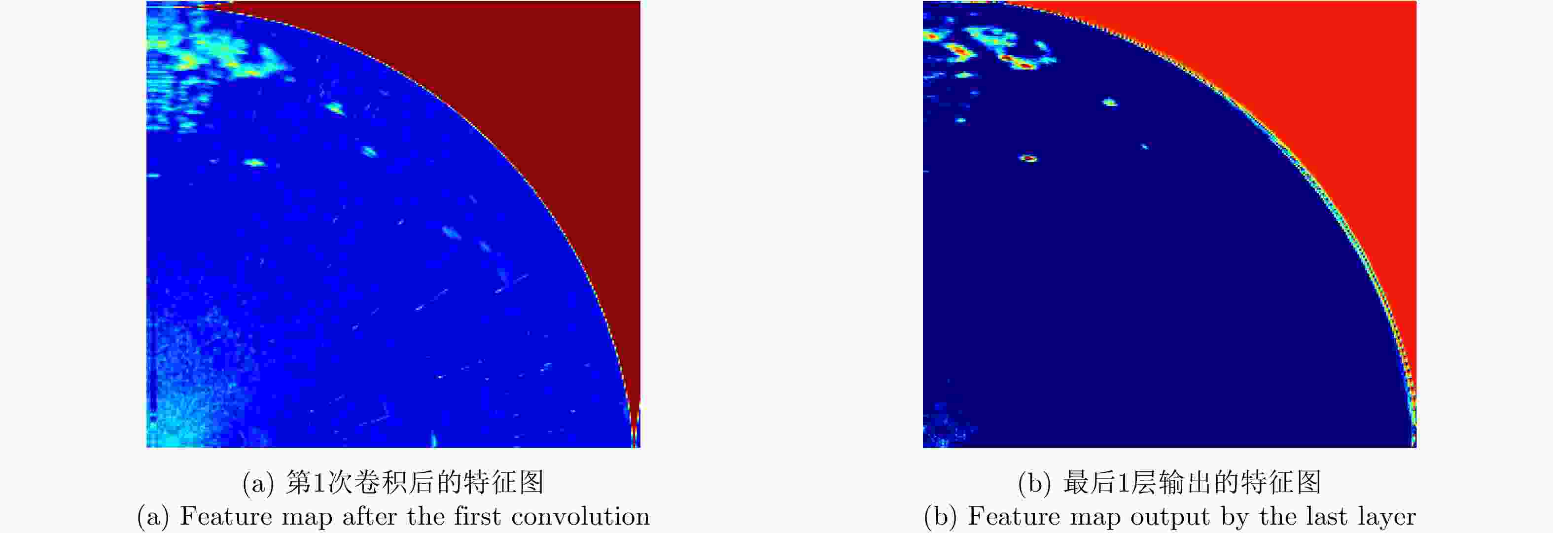
    图  6  Part Ⅰ 杂波抑制网络的部分特征图

    Figure  6.  Feature maps of the clutter suppression network in Part Ⅰ

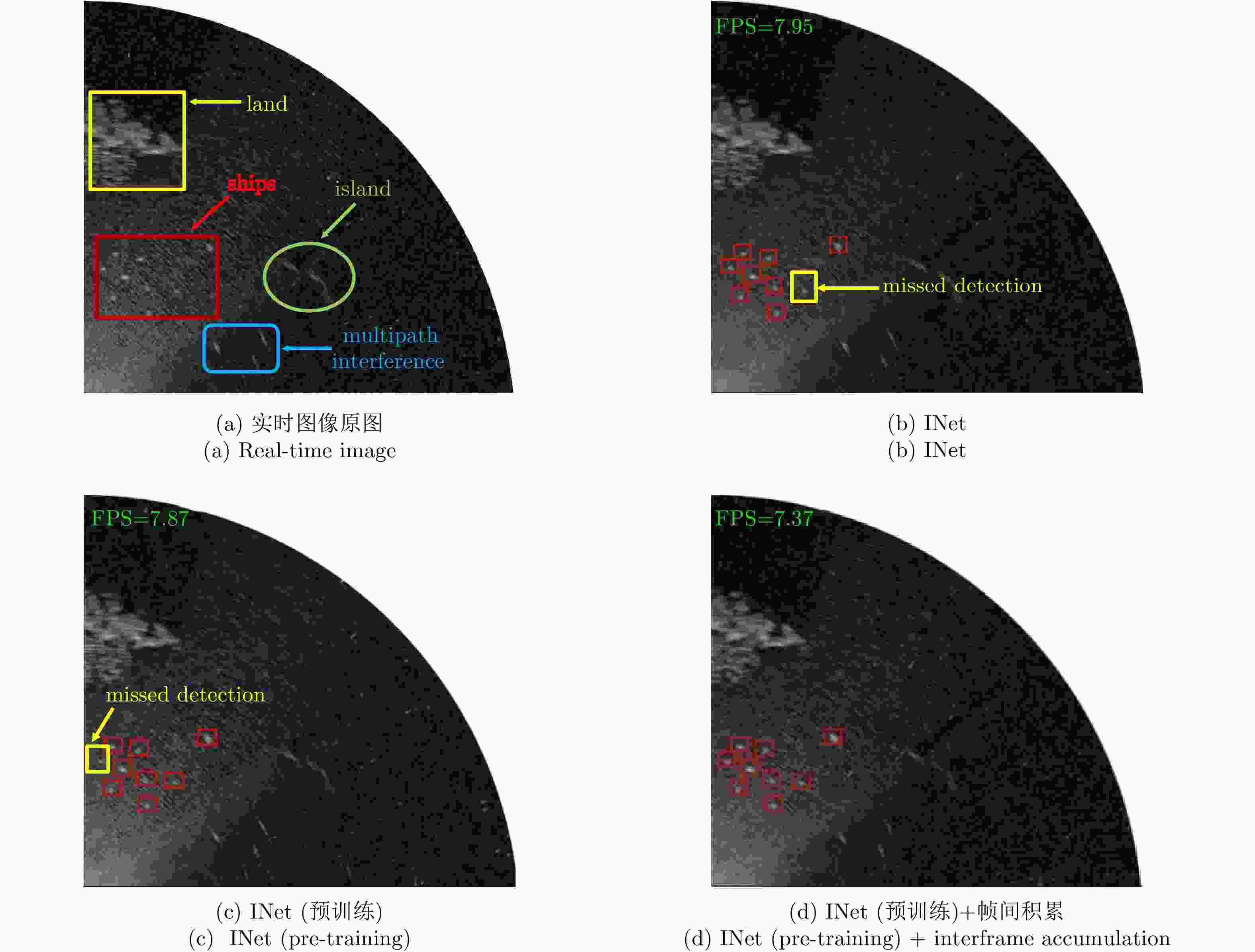
    图  7  模型优化前后的对比(Data_03#)

    Figure  7.  Comparison before and after model optimization (Data_03#)

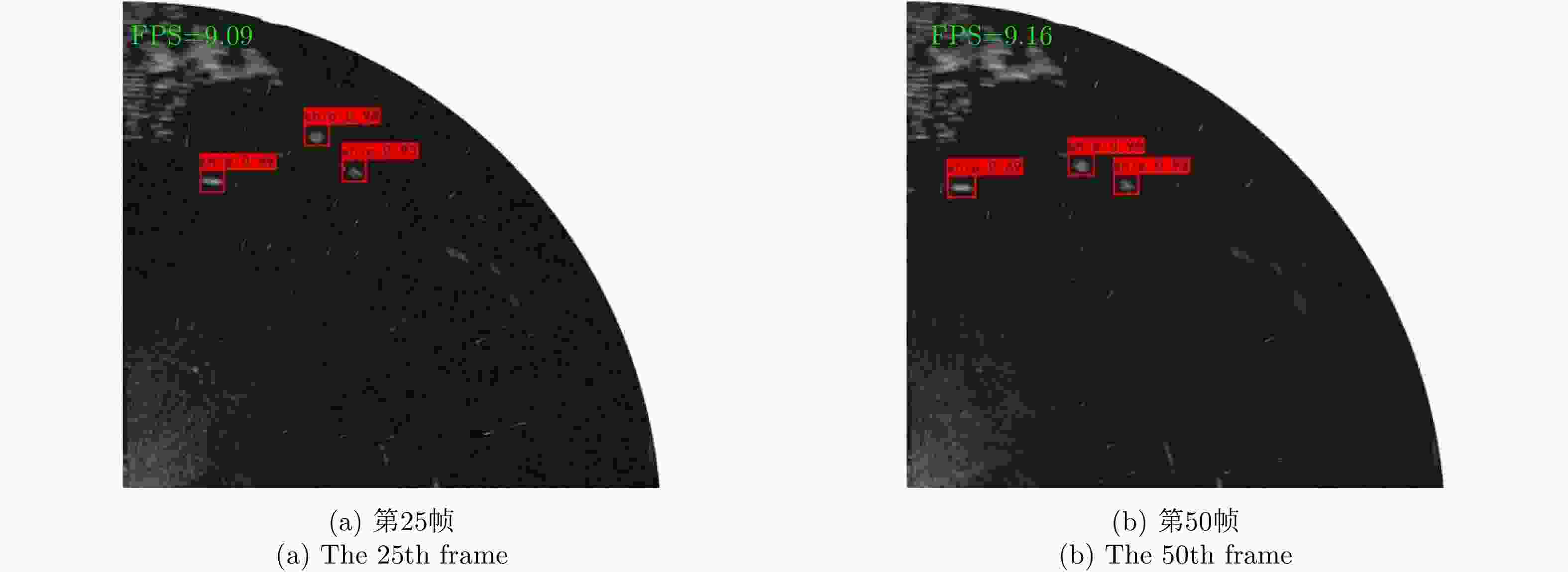
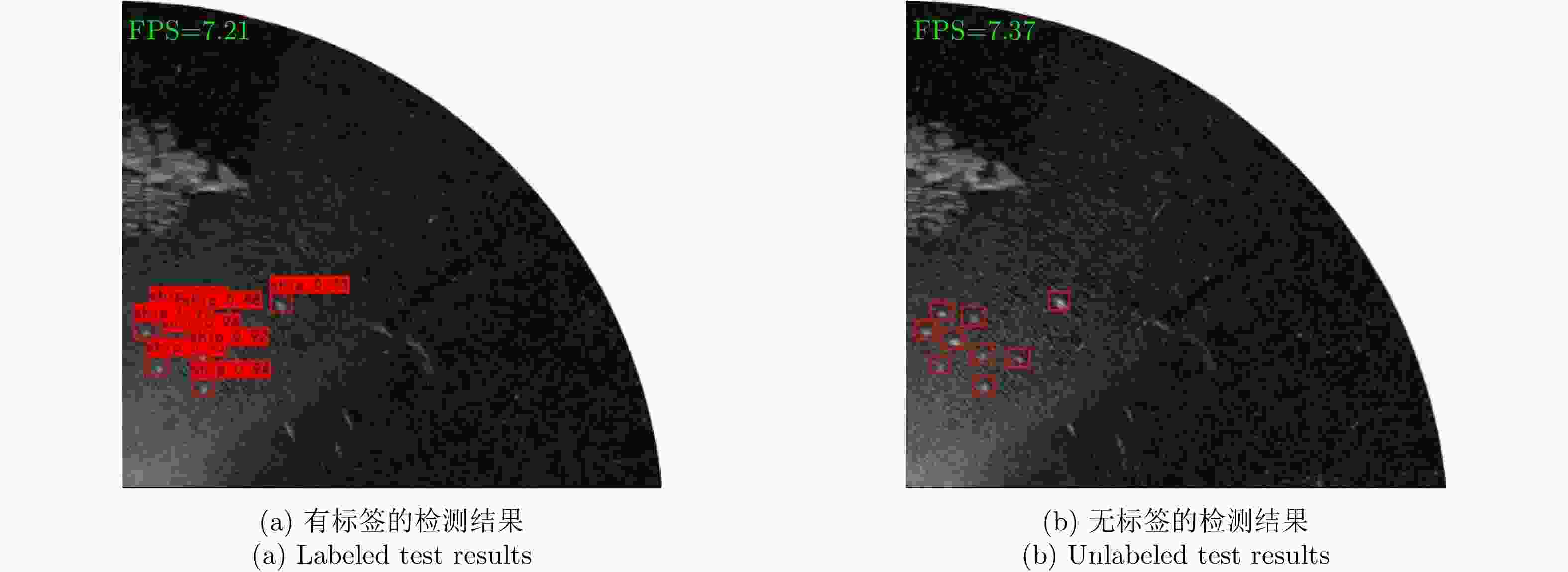
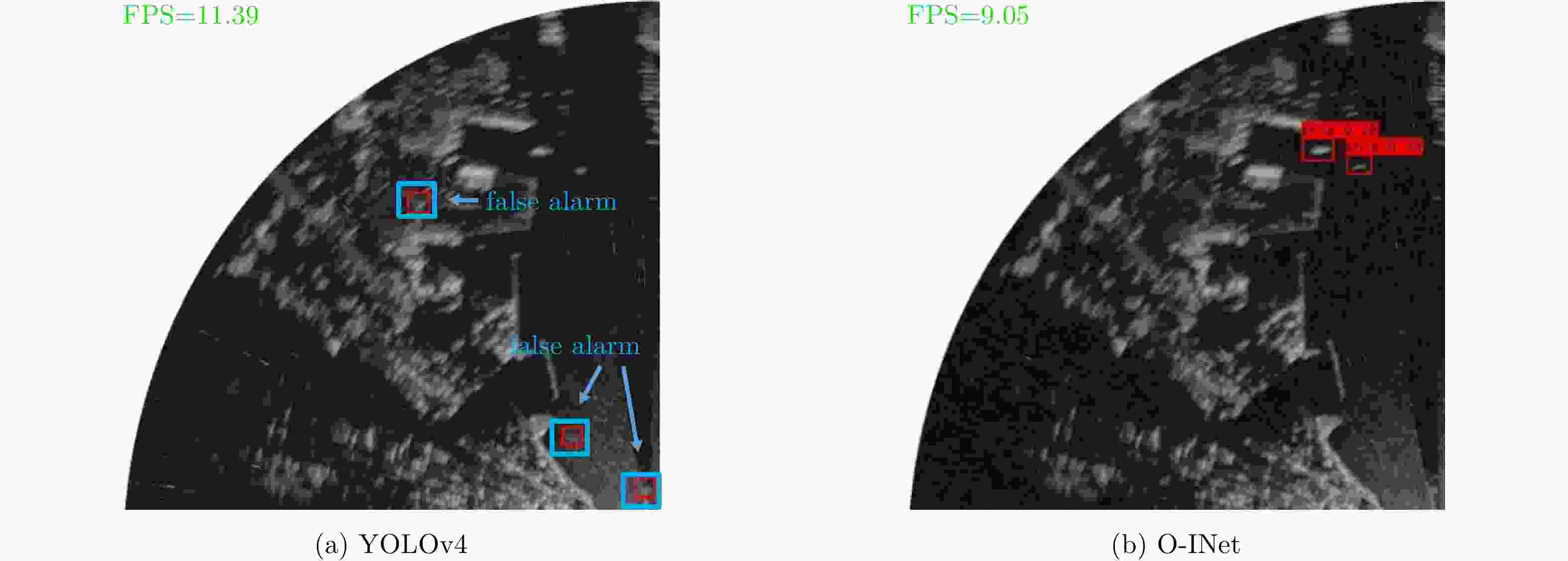
    图  8  低海况简单背景下的动目标(Data_01#)检测

    Figure  8.  Moving target detection under simple background of low sea state (Data_01#)

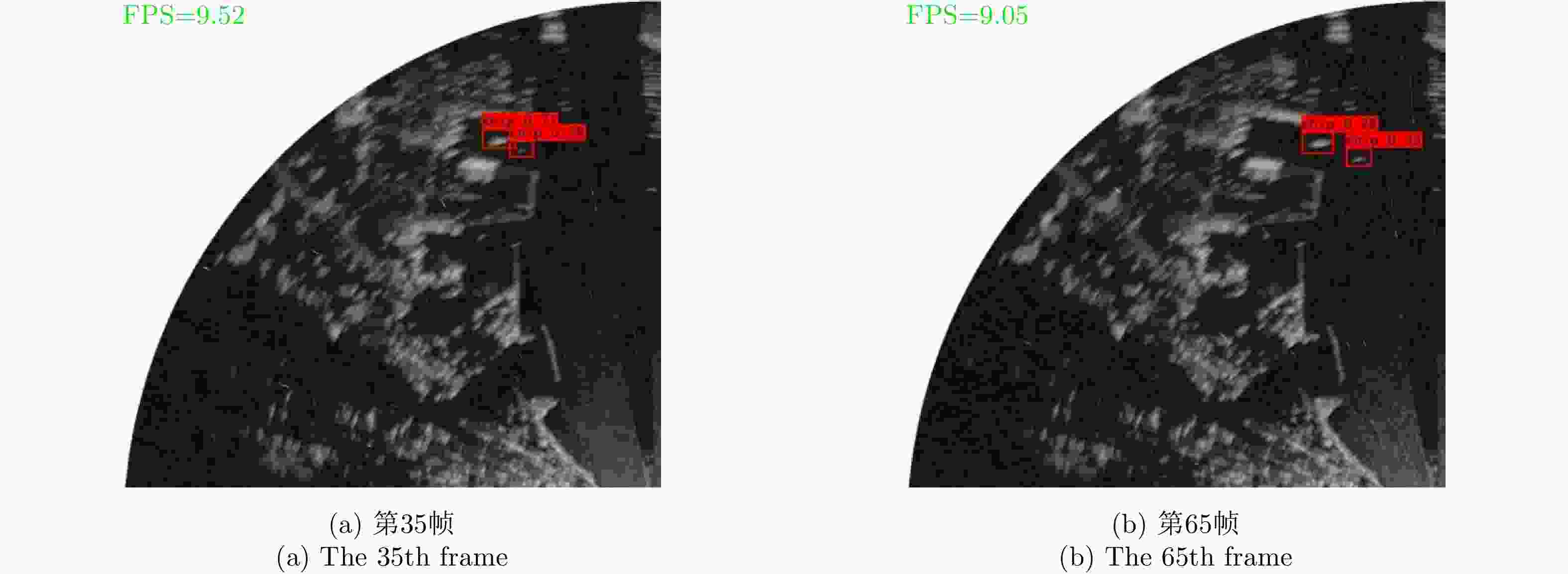
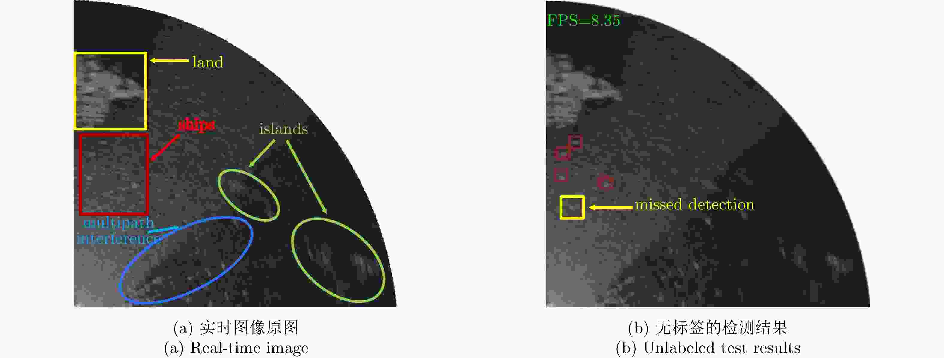
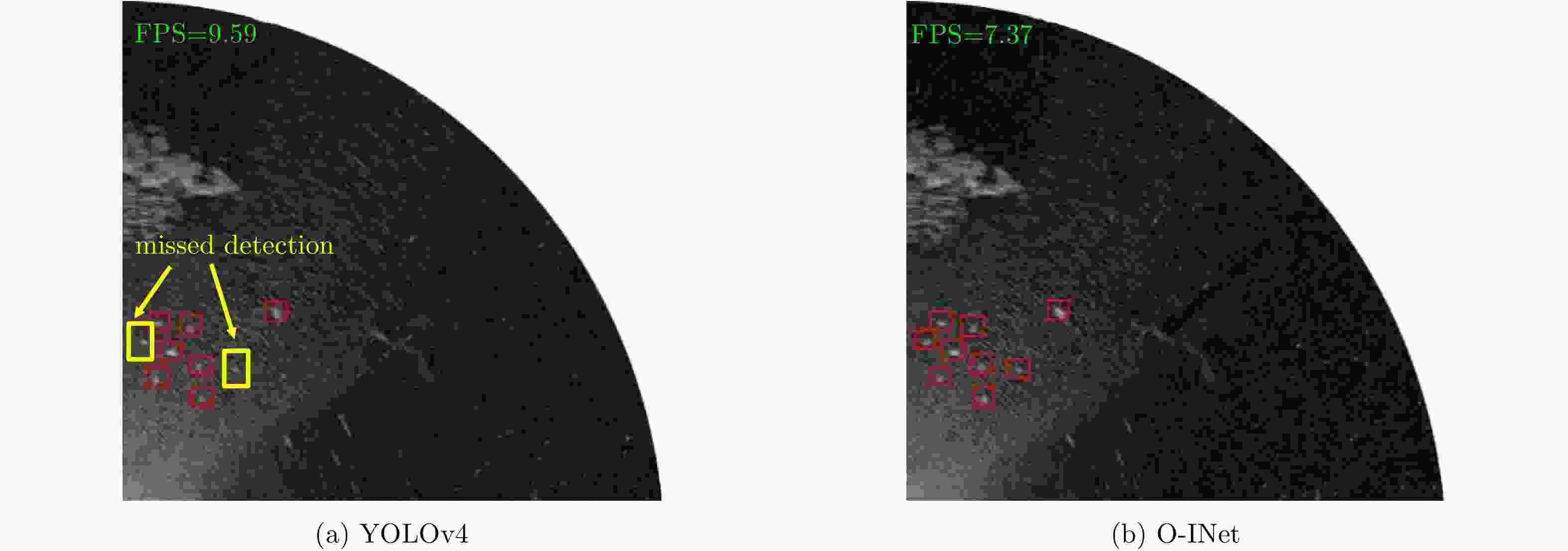
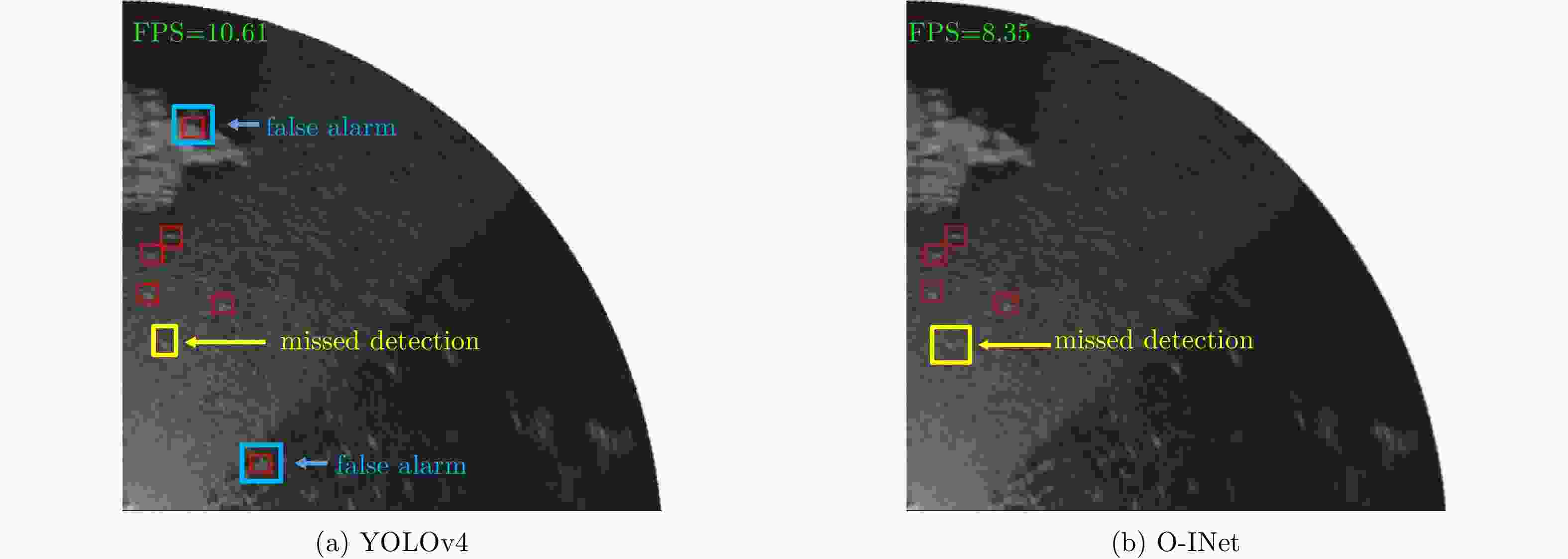
    图  9  低海况复杂背景下的动目标(Data_02#)检测

    Figure  9.  Moving target detection under complex background of low sea state (Data_02#)

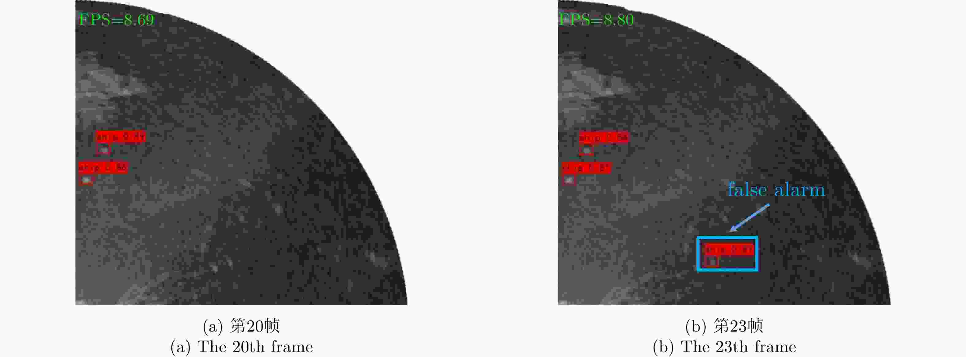
    图  10  高海况下的多目标(Data_03#)检测

    Figure  10.  Multi-target detection under high sea conditions (Data_03#)

    图  11  大雪下的多目标(Data_04#)检测

    Figure  11.  Multi-target detection under heavy snow (Data_04#)

    图  12  中雨下的多目标(Data_05#)检测结果对比

    Figure  12.  Comparison of multi-target detection results under rain weather (Data_05#)

    图  13  低海况简单背景下的动目标(Data_01#)检测结果对比

    Figure  13.  Comparison of moving targets under simple background of low sea state (Data_01#)

    图  14  低海况复杂背景下的动目标(Data_02#)检测结果对比

    Figure  14.  Moving target detection under complex background of low sea state (Data_02#)

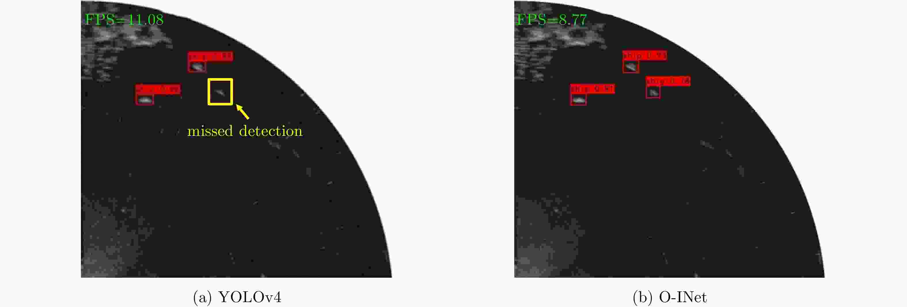
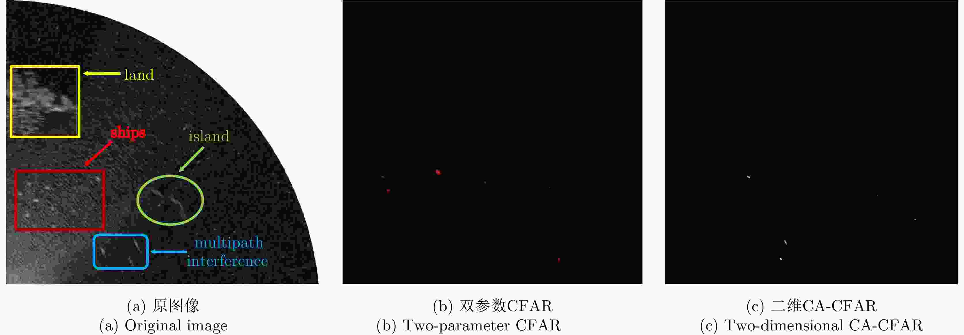
    图  15  高海况下的多目标(Data_03#)检测结果对比

    Figure  15.  Multi-target detection under high sea conditions (Data_03#)

    图  16  大雪下的多目标(Data_04#)检测结果对比

    Figure  16.  Multi-target detection under heavy snow (Data_04#)

    图  17  中雨下的动目标(Data_05#)检测结果对比

    Figure  17.  Comparison of multi-target detection results under rain weather (Data_05#)

    图  18  高海况下的多目标(Data_03#)检测结果

    Figure  18.  Multi-target detection results under high sea conditions (Data_03#)

    表  1  实时验证数据集参数

    Table  1.   Parameters of real-time verification dataset

    数据编号目标数量目标尺度目标速度海况背景PPI视频帧数
    Data_01#3中型船中速2级海杂波较弱150
    Data_02#2中、小型船低速2级地杂波较弱150
    Data_03#9中、小型船低速4级海杂波较强50
    Data_04#5中、小型船低速4级大雪50
    Data_05#2中、小型船低速4级中雨50
    下载: 导出CSV

    表  2  测试结果

    Table  2.   Test result

    算法RecallFA速度
    INet91.12%1.30%9.12 FPS
    下载: 导出CSV

    表  3  INet模型优化结果对比

    Table  3.   Comparison of optimization results

    算法简称Recall (%)FA (%)平均速度(FPS)
    INetINet91.121.129.12
    INet(预训练)\92.270.379.04
    INet +帧间积累\91.550.599.03
    INet (预训练)
    +帧间积累
    O-INet92.730.338.79
    下载: 导出CSV

    表  4  各类算法的实验结果对比

    Table  4.   Comparison of experimental results on different algorithms

    算法简称Recall(%)FA(%)平均速度(FPS)
    INet (ours)INet91.121.129.12
    INet (预训练)+帧间积累 (ours)O-INet92.730.338.79
    YOLOv3(预训练)[14]YOLOv383.234.059.25
    YOLOv4(预训练)[15]YOLOv489.042.7111.06
    下载: 导出CSV

    表  5  对测试集的检测结果(%)

    Table  5.   Test results about the test dataset (%)

    方法Pfa=10–4Pfa=10–3Pfa=10–2
    非相参积累+双参数CFAR16.9442.5257.71
    非相参积累+二维 CA-CFAR18.2537.7654.29
    O-INet80.9891.0493.65
    下载: 导出CSV
  • [1] 何友, 关键, 孟祥伟. 雷达目标检测与恒虚警处理[M]. 2版. 北京: 清华大学出版社, 2011: 1–15.

    HE You, GUAN Jian, and MENG Xiangwei. Radar Target Detection and CFAR Processing[M]. 2nd ed. Beijing: Tsinghua University Press, 2011: 1–15.
    [2] 黄勇, 陈小龙, 关键. 实测海尖峰特性分析及抑制方法[J]. 雷达学报, 2015, 4(3): 334–342. doi: 10.12000/JR14108

    HUANG Yong, CHEN Xiaolong, and GUAN Jian. Property analysis and suppression method of real measured sea spikes[J]. Journal of Radars, 2015, 4(3): 334–342. doi: 10.12000/JR14108
    [3] TRUNK G V and GEORGE S F. Detection of targets in non-Gaussian sea clutter[J]. IEEE Transactions on Aerospace and Electronic Systems, 1970, AES-6(5): 620–628. doi: 10.1109/TAES.1970.310062
    [4] 刘宁波, 董云龙, 王国庆, 等. X波段雷达对海探测试验与数据获取[J]. 雷达学报, 2019, 8(5): 656–667. doi: 10.12000/JR19089

    LIU Ningbo, DONG Yunlong, WANG Guoqing, et al. Sea-detecting X-band radar and data acquisition program[J]. Journal of Radars, 2019, 8(5): 656–667. doi: 10.12000/JR19089
    [5] YU Xiaohan, CHEN Xiaolong, HUANG Yong, et al. Fast detection method for low-observable maneuvering target via robust sparse fractional Fourier transform[J]. IEEE Geoscience and Remote Sensing Letters, 2020, 17(6): 978–982. doi: 10.1109/LGRS.2019.2939264
    [6] 许述文, 石星宇, 水鹏朗. 复合高斯杂波下抑制失配信号的自适应检测器[J]. 雷达学报, 2019, 8(3): 326–334. doi: 10.12000/JR19030

    XU Shuwen, SHI Xingyu, and SHUI Penglang. An adaptive detector with mismatched signals rejection in compound Gaussian clutter[J]. Journal of Radars, 2019, 8(3): 326–334. doi: 10.12000/JR19030
    [7] LIU Yi, ZHANG Shufang, SUO Jidong, et al. Research on a new Comprehensive CFAR (Comp-CFAR) processing method[J]. IEEE Access, 2019, 7: 19401–19413. doi: 10.1109/ACCESS.2019.2897358
    [8] WANG H and CAI L. A localized adaptive MTD processor[J]. IEEE Transactions on Aerospace and Electronic Systems, 1991, 27(3): 532–539. doi: 10.1109/7.81435
    [9] CHEN Xiaolong, GUAN Jian, WANG Guoqing, et al. Fast and refined processing of radar maneuvering target based on hierarchical detection via sparse fractional representation[J]. IEEE Access, 2019, 7: 149878–149889. doi: 10.1109/ACCESS.2019.2947169
    [10] CHEN Xiaolong, YU Xiaohan, HUANG Yong, et al. Adaptive clutter suppression and detection algorithm for radar maneuvering target with high-order motions via sparse fractional ambiguity function[J]. IEEE Journal of Selected Topics in Applied Earth Observations and Remote Sensing, 2020, 13: 1515–1526. doi: 10.1109/JSTARS.2020.2981046
    [11] 王俊, 郑彤, 雷鹏, 等. 深度学习在雷达中的研究综述[J]. 雷达学报, 2018, 7(4): 395–411. doi: 10.12000/JR18040

    WANG Jun, ZHENG Tong, LEI Peng, et al. Study on deep learning in radar[J]. Journal of Radars, 2018, 7(4): 395–411. doi: 10.12000/JR18040
    [12] 牟效乾, 陈小龙, 苏宁远, 等. 基于时频图深度学习的雷达动目标检测与分类[J]. 太赫兹科学与电子信息学报, 2019, 17(1): 105–111. doi: 10.11805/TKYDA201901.0105

    MOU Xiaoqian, CHEN Xiaolong, SU Ningyuan, et al. Radar detection and classification of moving target using deep convolutional neural networks on time-frequency graphs[J]. Journal of Terahertz Science and Electronic Information Technology, 2019, 17(1): 105–111. doi: 10.11805/TKYDA201901.0105
    [13] REN Shaoqing, HE Kaiming, GIRSHICK R, et al. Faster R-CNN: Towards real-time object detection with region proposal networks[J]. IEEE Transactions on Pattern Analysis and Machine Intelligence, 2015, 39(6): 1137–1149. doi: 10.1109/TPAMI.2016.2577031
    [14] REDMON J and FARHADI A. YOLOv3: An incremental improvement[EB/OL]. https://arxiv.org/abs/1804.02767, 2018.
    [15] BOCHKOVSKIY A, WANG C Y, and LIAO H Y M. YOLOv4: Optimal speed and accuracy of object detection[EB/OL]. https://arxiv.org/abs/2004.10934,2020.
    [16] 杜兰, 王兆成, 王燕, 等. 复杂场景下单通道SAR目标检测及鉴别研究进展综述[J]. 雷达学报, 2020, 9(1): 34–54. doi: 10.12000/JR19104

    DU Lan, WANG Zhaocheng, WANG Yan, et al. Survey of research progress on target detection and discrimination of single-channel SAR images for complex scenes[J]. Journal of Radars, 2020, 9(1): 34–54. doi: 10.12000/JR19104
    [17] 苏宁远, 陈小龙, 陈宝欣, 等. 雷达海上目标双通道卷积神经网络特征融合智能检测方法[J]. 现代雷达, 2019, 41(10): 47–52, 57. doi: 10.16592/j.cnki.1004-7859.2019.10.009

    SU Ningyuan, CHEN Xiaolong, CHEN Baoxin, et al. Dual-channel convolutional neural networks feature fusion method for radar maritime target intelligent detection[J]. Modern Radar, 2019, 41(10): 47–52, 57. doi: 10.16592/j.cnki.1004-7859.2019.10.009
    [18] 苏宁远, 陈小龙, 关键, 等. 基于卷积神经网络的海上微动目标检测与分类方法[J]. 雷达学报, 2018, 7(5): 565–574. doi: 10.12000/JR18077

    SU Ningyuan, CHEN Xiaolong, GUAN Jian, et al. Detection and classification of maritime target with micro-motion based on CNNs[J]. Journal of Radars, 2018, 7(5): 565–574. doi: 10.12000/JR18077
    [19] CHEN Chen, HE Chuan, HU Changhua, et al. MSARN: A deep neural network based on an adaptive recalibration mechanism for multiscale and arbitrary-oriented SAR ship detection[J]. IEEE Access, 2019, 7: 159262–159283. doi: 10.1109/ACCESS.2019.2951030
    [20] 黄洁, 姜志国, 张浩鹏, 等. 基于卷积神经网络的遥感图像舰船目标检测[J]. 北京航空航天大学学报, 2017, 43(9): 1841–1848. doi: 10.13700/j.bh.1001-5965.2016.0755

    HUANG Jie, JIANG Zhiguo, ZHANG Haopeng, et al. Ship object detection in remote sensing images using convolutional neural networks[J]. Journal of Beijing University of Aeronautics and Astronautics, 2017, 43(9): 1841–1848. doi: 10.13700/j.bh.1001-5965.2016.0755
    [21] WEI Xiukun, WEI Dehua, SUO Da, et al. Multi-target defect identification for railway track line based on image processing and improved YOLOv3 model[J]. IEEE Access, 2020, 8: 61973–61988. doi: 10.1109/ACCESS.2020.2984264
    [22] XIAO Dong, SHAN Feng, LI Ze, et al. A target detection model based on improved Tiny-Yolov3 under the environment of mining truck[J]. IEEE Access, 2019, 7: 123757–123764. doi: 10.1109/ACCESS.2019.2928603
    [23] ZHANG Huibing, QIN Longfei, LI Jun, et al. Real-time detection method for small traffic signs based on Yolov3[J]. IEEE Access, 2020, 8: 64145–64156. doi: 10.1109/ACCESS.2020.2984554
    [24] BA J L, KIROS J R, and HINTON G E. Layer normalization[EB/OL]. https://arxiv.org/abs/1607.06450, 2016.
    [25] WANG C Y, LIAO H Y M, YEH I H, et al. CSPNet: A new backbone that can enhance learning capability of CNN[EB/OL]. https://arxiv.org/abs/1911.11929,2019.
    [26] HE Kaiming, ZHANG Xiangyu, REN Shaoqing, et al. Deep residual learning for image recognition[C]. 2016 IEEE Conference on Computer Vision and Pattern Recognition (CVPR), Las Vegas, USA, 2016: 770–778. doi: 10.1109/CVPR.2016.90.
    [27] AI Jiaqiu, YANG Xuezhi, DONG Zhangyu, et al. A new two parameter CFAR ship detector in Log-Normal clutter[C]. 2017 IEEE Radar Conference (RadarConf), Seattle, USA, 2017: 195–199. doi: 10.1109/RADAR.2017.7944196.
    [28] YANG Jianyu, LU Chao, and LI Liangchao. Target detection in passive millimeter wave image based on two-dimensional cell-weighted average CFAR[C]. The IEEE 11th International Conference on Signal Processing, Beijing, China, 2012: 917–921. doi: 10.1109/ICoSP.2012.6491729.
  • 期刊类型引用(4)

    1. 葛津津,周浩,凌天庆. 一种应用于脉冲探地雷达前端的探测子系统. 电子测量技术. 2022(04): 27-32 . 百度学术
    2. 尹诗,郭伟. 用于探地雷达的超宽带天线设计与仿真. 电子设计工程. 2018(03): 98-102 . 百度学术
    3. 宋立伟,张超,洪涛. 冲击波载荷对平面阵列天线电性能的影响. 电子机械工程. 2017(04): 1-5+58 . 百度学术
    4. 尹德,叶盛波,刘晋伟,纪奕才,刘小军,方广有. 一种用于高速公路探地雷达的新型时域超宽带TEM喇叭天线. 雷达学报. 2017(06): 611-618 . 本站查看

    其他类型引用(6)

  • 加载中
图(18) / 表(5)
计量
  • 文章访问数: 5048
  • HTML全文浏览量: 1899
  • PDF下载量: 584
  • 被引次数: 10
出版历程
  • 收稿日期:  2020-07-02
  • 修回日期:  2020-08-16
  • 网络出版日期:  2020-08-28

目录

/

返回文章
返回