
 作者中心
作者中心 专家审稿
专家审稿 责编办公
责编办公 编辑办公
编辑办公
Review of On-orbit State Estimation of Space Targets with Radar Imagery(in English)
-
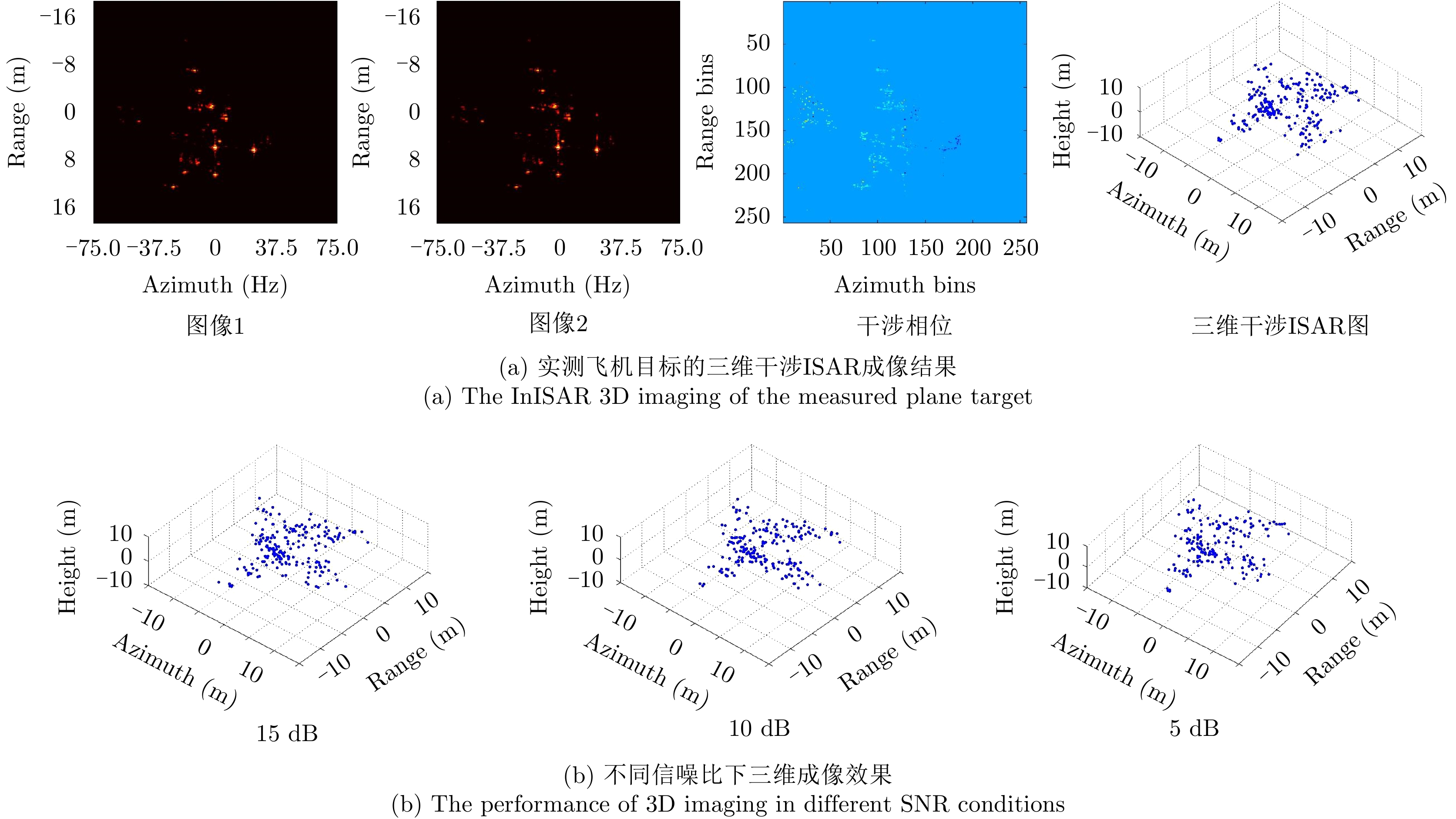
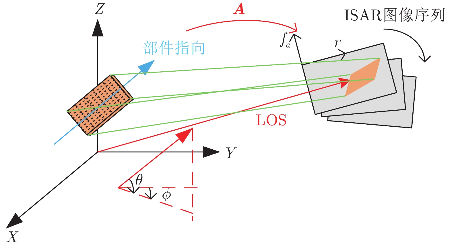
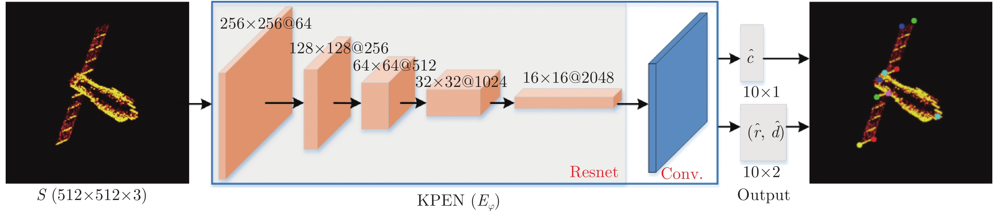
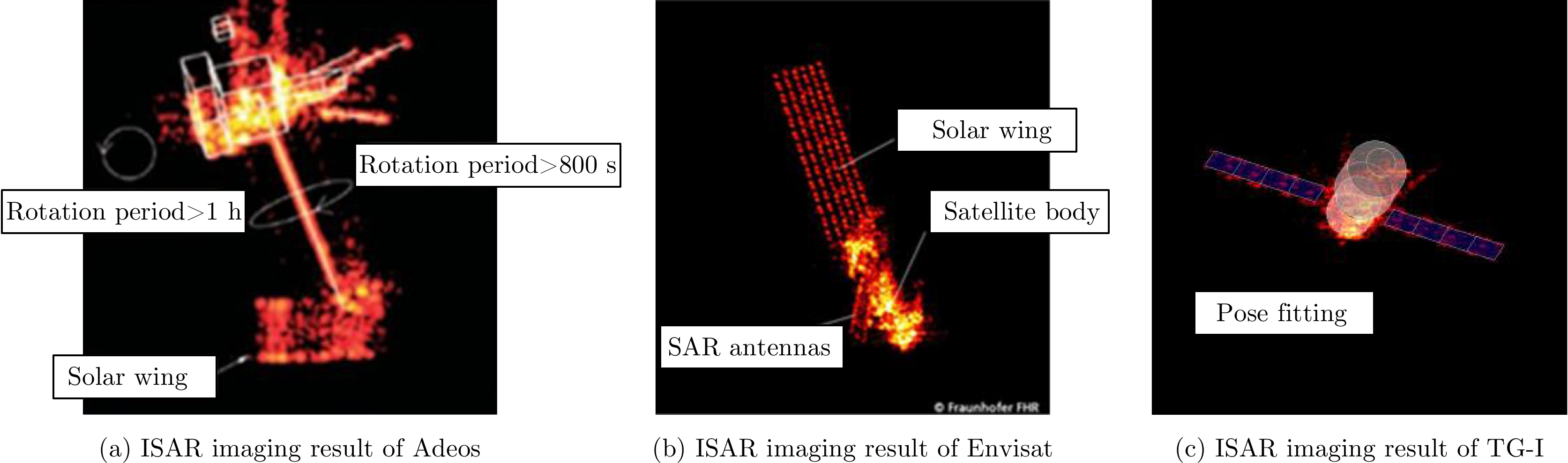
摘要: 空间目标状态估计旨在获取目标在轨姿态运动和几何结构等状态参数,是完成目标动作意图分析、排查潜在故障威胁和预判在轨态势等任务的关键技术。通过雷达光电成像信息处理实现在轨姿态估计是空间目标状态分析的重要途径,当前已经形成了一系列代表性实用方法。该文首先简要介绍了国内外用于空间目标监测的地基逆合成孔径雷达发展现状;重点针对空间目标时序特征匹配、三维成像重建和多视融合姿态估计多类代表性方法进行原理介绍与技术总结:数据特征匹配的状态估计性能可靠但依赖目标模型先验;三维几何重建的状态估计具备目标精细刻画潜力但观测几何要求高。同时,该文也对空间目标在轨状态估计方向未来发展趋势进行了展望。Abstract: Space target state estimation aims to obtain a target’s on-orbit attitude, structure, movement, and other parameters accurately. This process helps observers analyze the target action intention, check for potential fault threats, and predict the development of on-orbit situations and is the core technology in the field of space situation awareness. Currently, the estimation of the on-orbit state of space targets mainly relies on external observations from high-performance sensors, such as radars, paralleled by the emergence of a series of representative methods. This paper briefly introduces the development status of inverse synthetic-aperture radar used for space target monitoring at home and abroad. Then, several representative methods, including data feature matching, three-dimensional (3D) imaging reconstruction, and multi-look fusion estimation, are introduced. The data feature-matching technology performs well when the priori target 3D model and scene conditions are given. The state estimation with 3D geometric reconstruction has the potential for fine description of the target, but high-level observation conditions are required. Finally, the future development trend of this direction is forecasted.
-
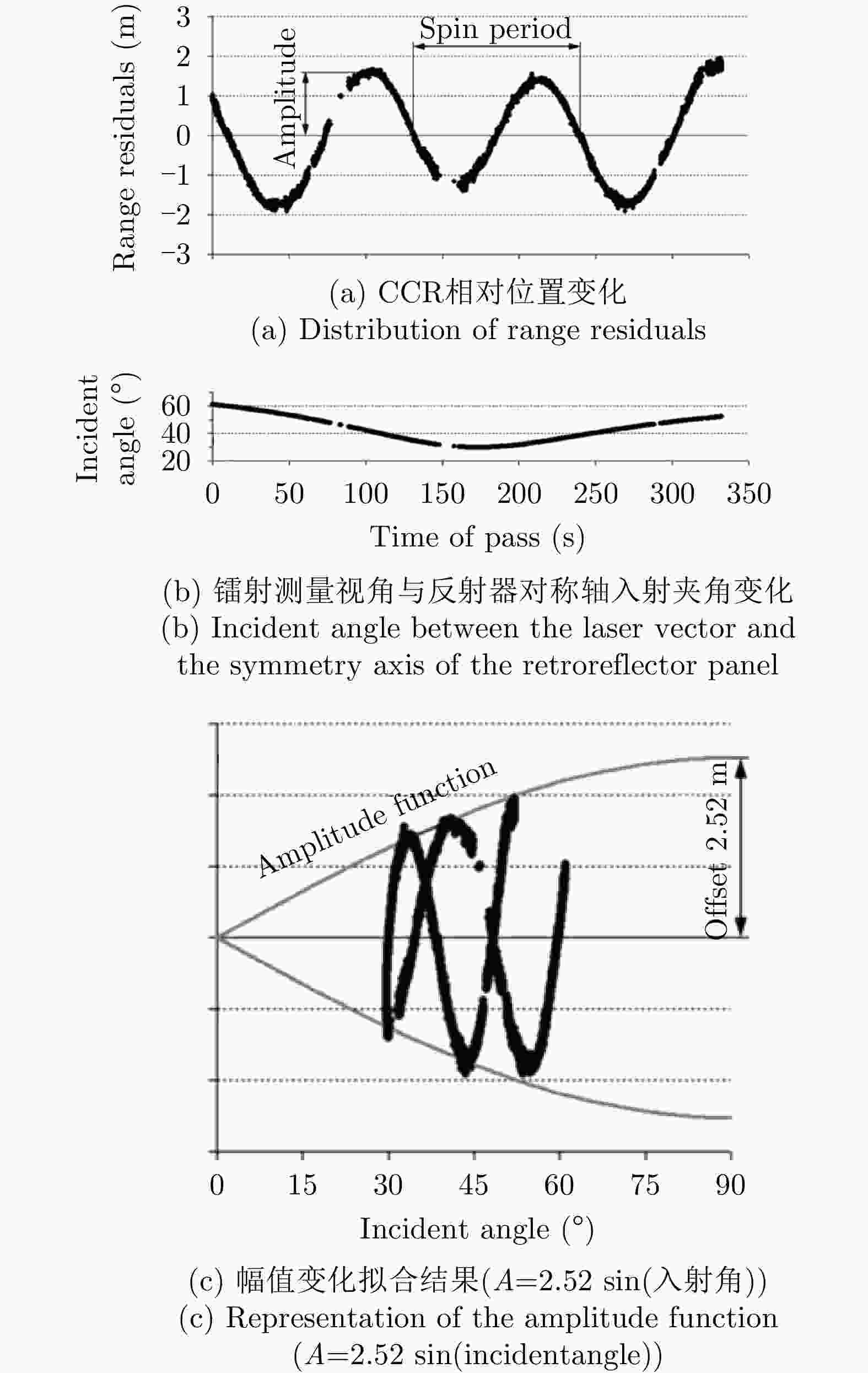

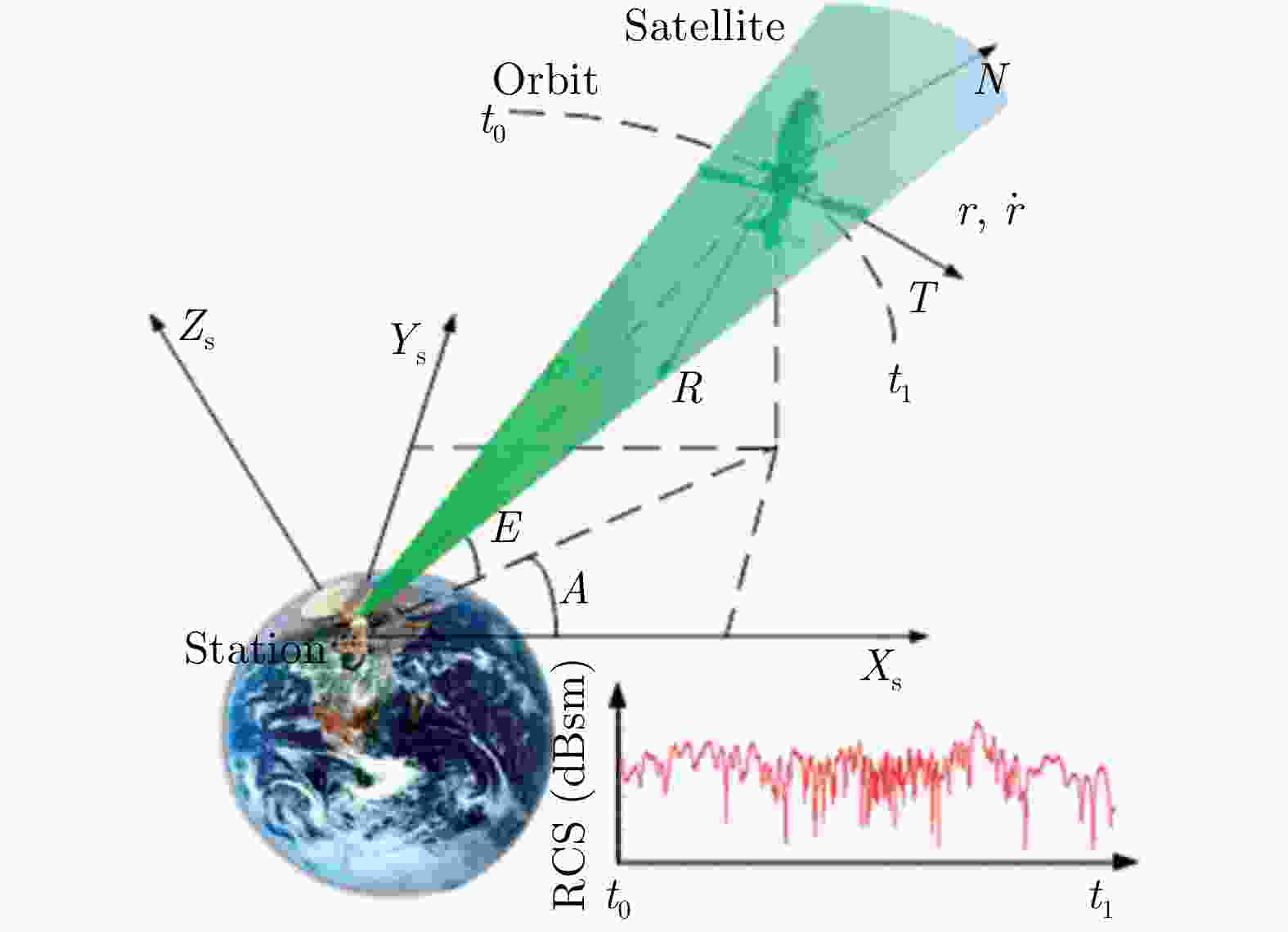
图 5 空间目标地基雷达RCS测量观测几何
Figure 5. RCS measuring geometry configuration of space targets via ground-based radar

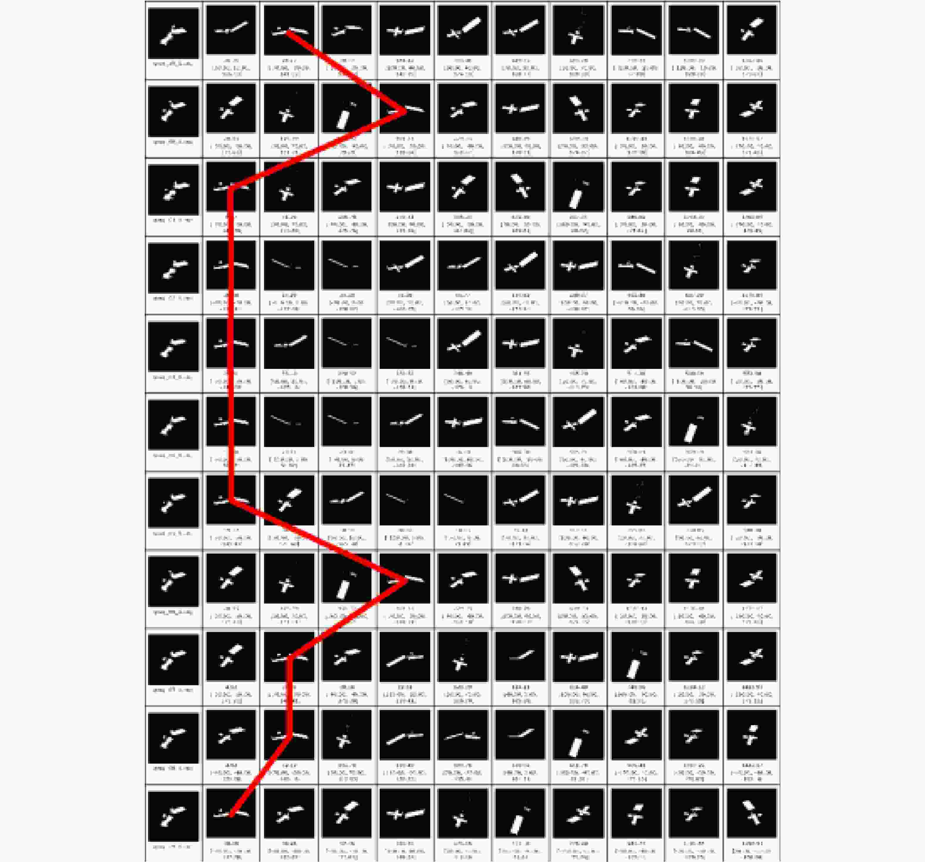
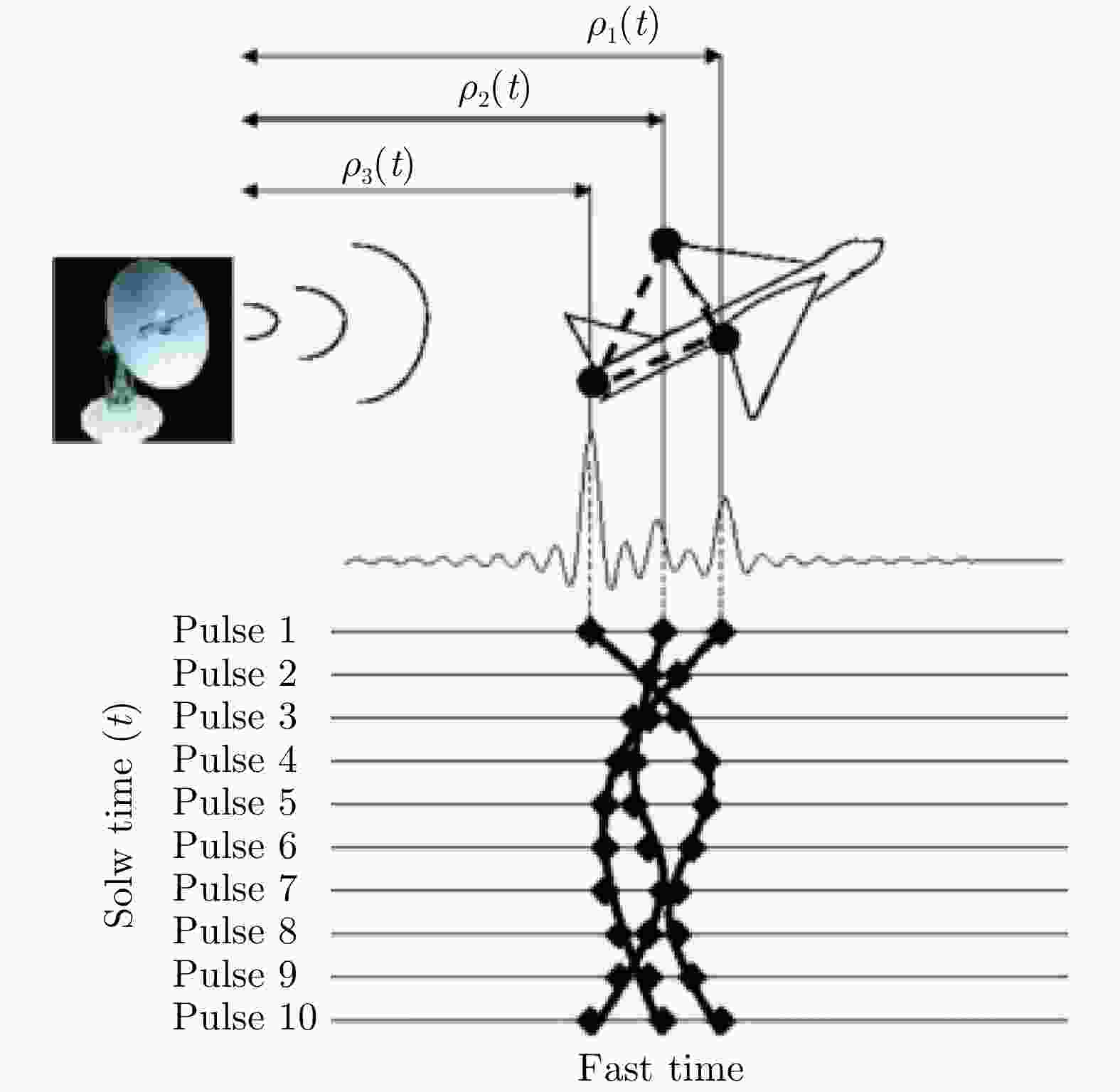

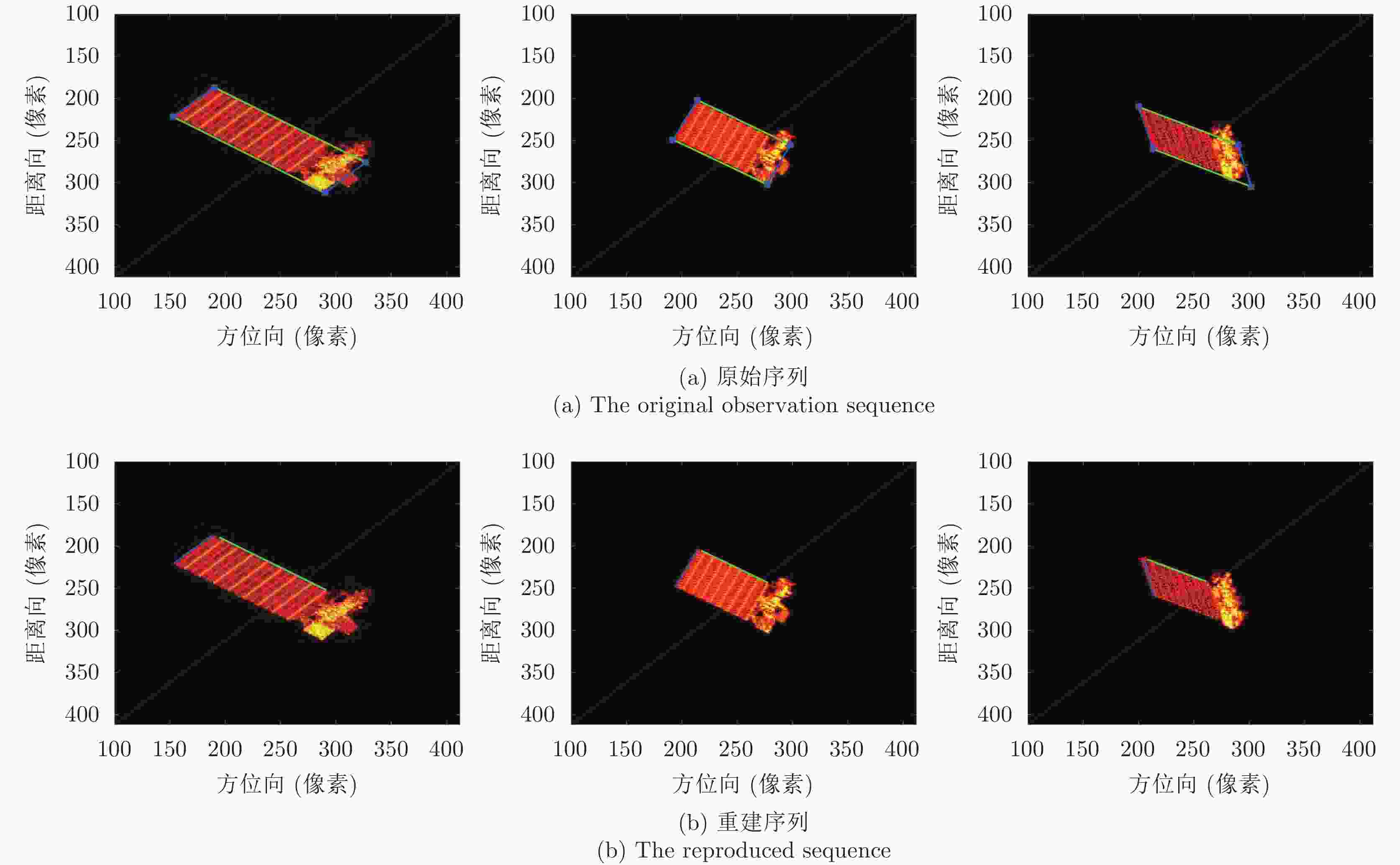

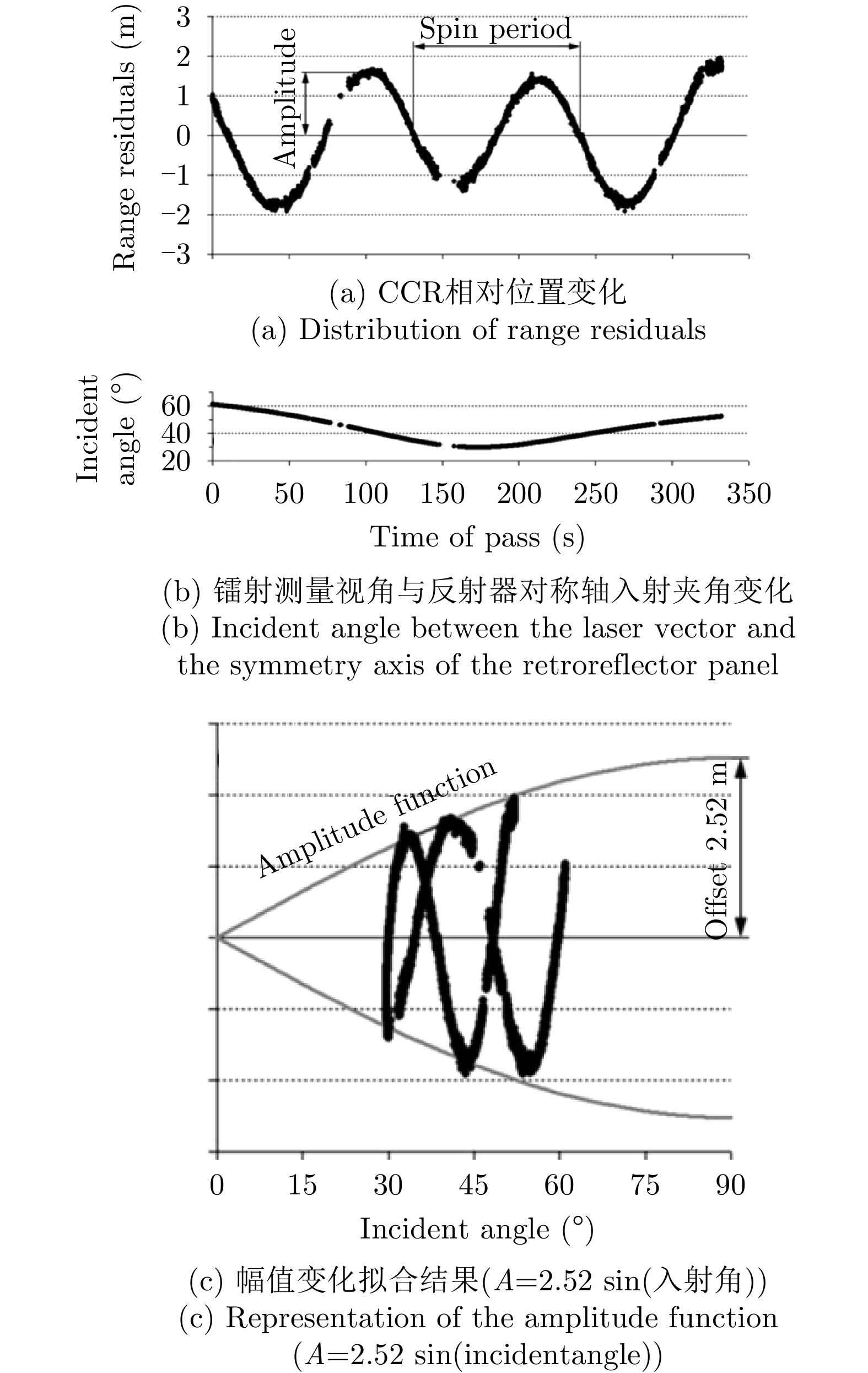
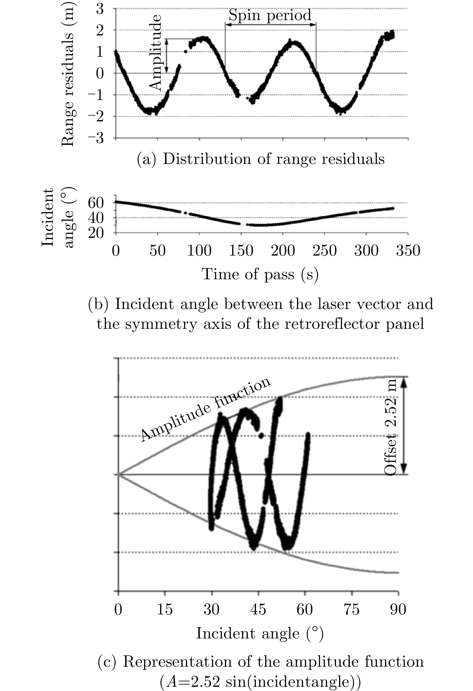
图 3 Range residuals calculated for Envisat pass measured by Graz SLR station on July 12, 2013[17]

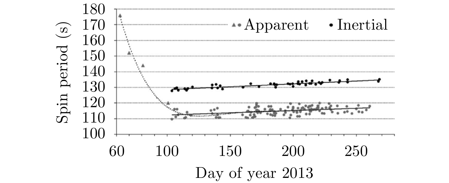
图 4 Spin period analysis of Envisat in 2013[17] (black points indicate an inertial spin period and gray points apparent spin period)

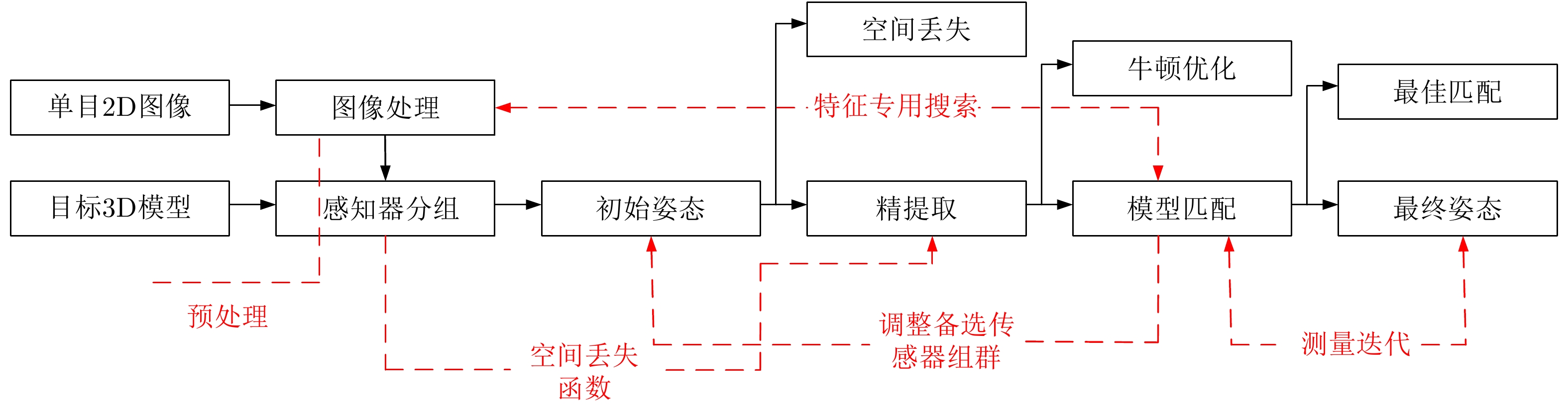
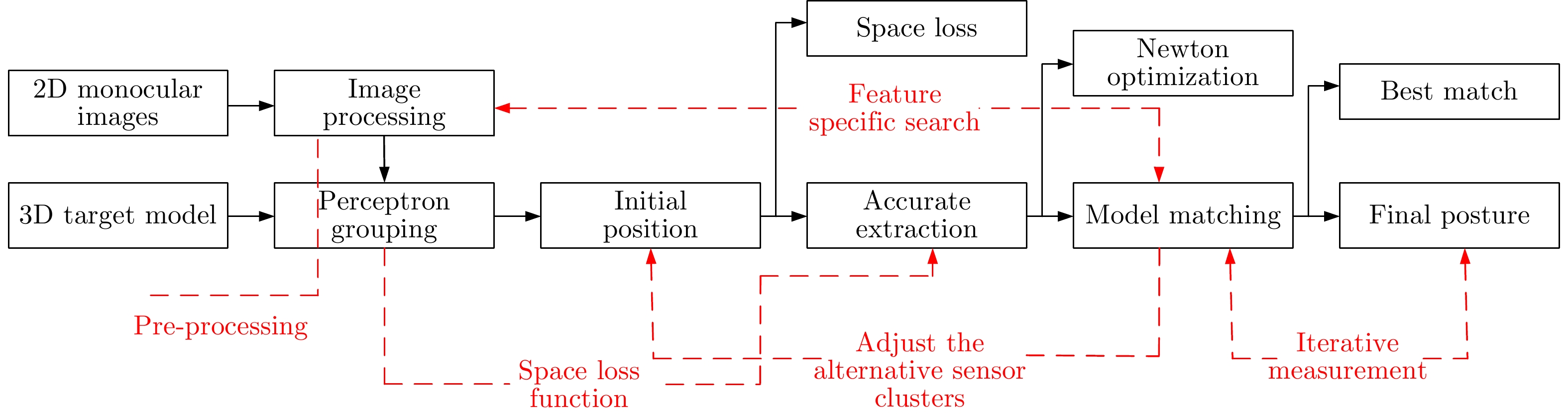
图 9 Attitude estimation for Envisat sequence frames after constraining the search space[28]

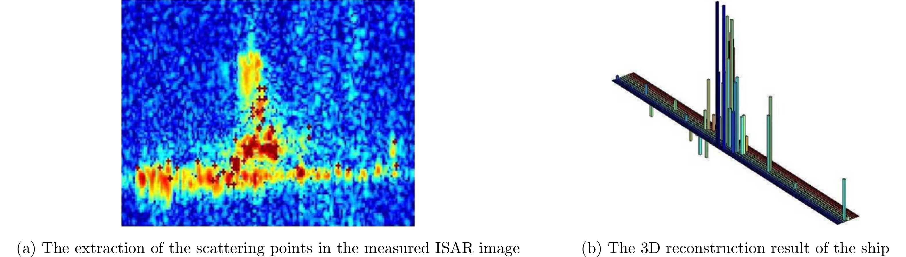
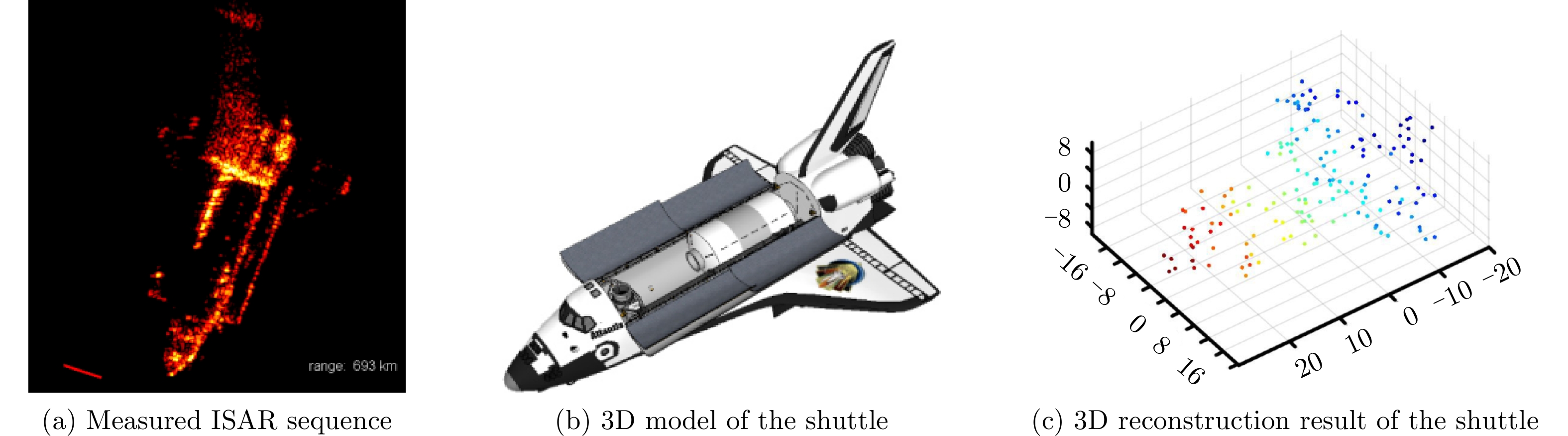
图 10 Recording the distance sequence of target scattering points through radar ranging[35]

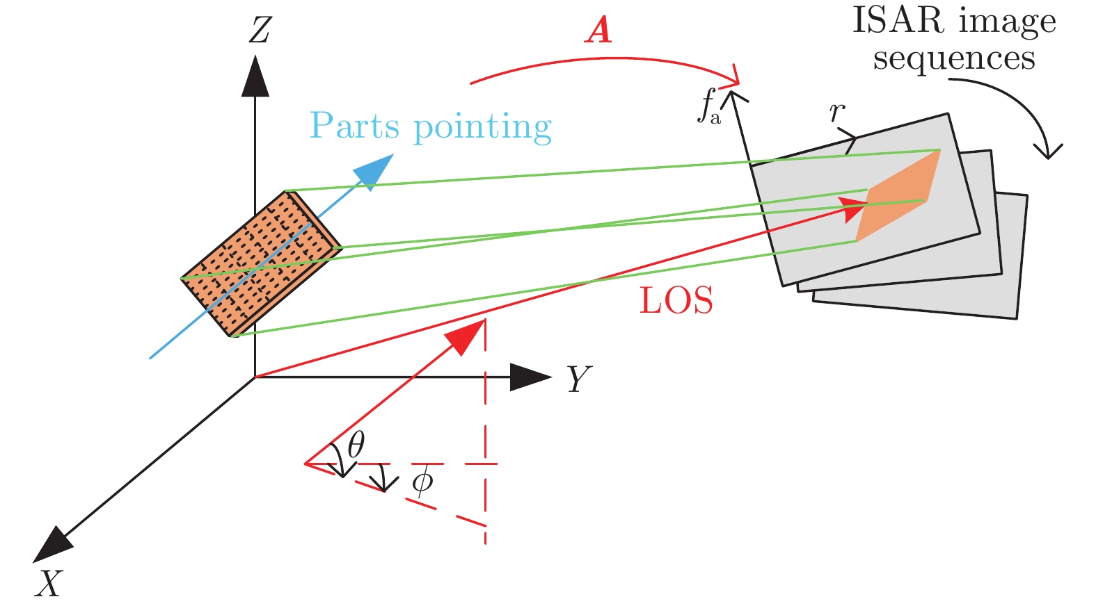
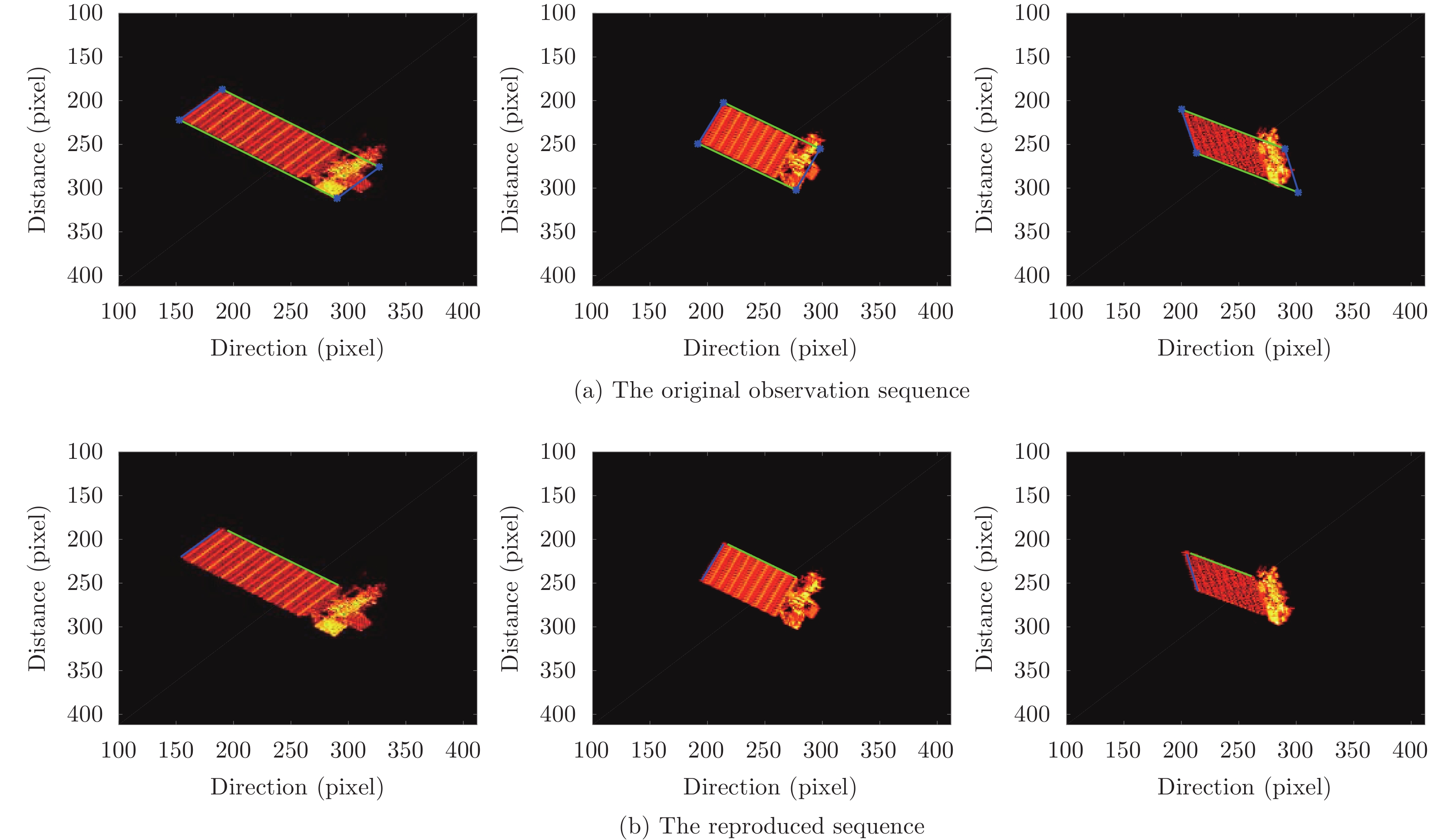
图 17 Comparison between the original observation sequence and the reproduced sequence with estimated attitude parameters[51]
-
[1] New Mexico State University. How many satellites in space[EB/OL]. https://web.nmsu.edu/~tnuslein/ICT460/SPECIAL/Page3.htm, 2021. [2] 央视网. 美俄卫星太空相撞[EB/OL]. http://news.cctv.com/special/satellitecrash/home/index.shtml, 2018. [3] Orbital debris quarterly news[R]. NASA Orbital Debris Program Office, 2010, 14(3). [4] 邢孟道, 林浩, 陈溅来, 等. 多平台合成孔径雷达成像算法综述[J]. 雷达学报, 2019, 8(6): 732–757. doi: 10.12000/JR19102XING Mengdao, LIN Hao, CHEN Jianlai, et al. A review of imaging algorithms in multi-platform-borne synthetic aperture radar[J]. Journal of Radars, 2019, 8(6): 732–757. doi: 10.12000/JR19102 [5] 马岩, 马驰, 解延浩, 等. 基于视频遥感卫星的空间目标光度测量[J]. 光子学报, 2019, 48(12): 1228002. doi: 10.3788/gzxb20194812.1228002MA Yan, MA Chi, XIE Yanhao, et al. Space target luminosity measurement based on video remote sensing satellites[J]. Acta Photonica Sinica, 2019, 48(12): 1228002. doi: 10.3788/gzxb20194812.1228002 [6] 王雪松, 陈思伟. 合成孔径雷达极化成像解译识别技术的进展与展望[J]. 雷达学报, 2020, 9(2): 259–276. doi: 10.12000/JR19109WANG Xuesong and CHEN Siwei. Polarimetric synthetic aperture radar interpretation and recognition: Advances and perspectives[J]. Journal of Radars, 2020, 9(2): 259–276. doi: 10.12000/JR19109 [7] 郭崇滨, 夏喜旺, 斯朝铭, 等. 分布式精密编队卫星相对位姿测量技术综述[J]. 航天控制, 2018, 36(6): 83–89. doi: 10.16804/j.cnki.issn1006-3242.2018.06.015GUO Chongbin, XIA Xiwang, SI Chaoming, et al. A survey of relative position and attitude measurement for formation flying satellite[J]. Aerospace Control, 2018, 36(6): 83–89. doi: 10.16804/j.cnki.issn1006-3242.2018.06.015 [8] AVENT R K, SHELTON J D, and BROWN P. The ALCOR C-band imaging radar[J]. IEEE Antennas and Propagation Magazine, 1996, 38(3): 16–27. doi: 10.1109/74.511949 [9] JAIN A and PATEL I. SAR/ISAR imaging of a nonuniformly rotating target[J]. IEEE Transactions on Aerospace and Electronic Systems, 1992, 28(1): 317–320. doi: 10.1109/7.135457 [10] BILL D. Wideband radar[J]. Lincoln Laboratory Journal, 2010, 18(2): 87–88. [11] CAMP W W, MAYHAN J T, and O’DONNELL R M. Wideband radar for ballistic missile defense and range-doppler imaging of satellites[J]. Lincoln Laboratory Journal, 2000, 12(2): 267–280. [12] MIT Lincoln Lab. The annual report summarizes lincoln laboratory[EB/OL]. https://archive.ll.mit.edu/publications/index.html, 2020. [13] Fraunhofer FHR Lab. Space observation radar TIRA[EB/OL]. https://www.fhr.fraunhofer.de/en/the-institute/technical-equipment/Space-observation-radar-TIRA.html, 2020. [14] VIRGILI B B, LEMMENS S, and KRAG H. Investigation on Envisat attitude motion[R]. Proceedings of the Deorbit Workshop, Noordwijk, The Netherlands, 2014. [15] Monitoring the re-entry of the Chinese space station Tiangong-1 with TIRA[EB/OL]. https://www.fhr.fraunhofer.de/en/businessunits/space/monitoring-the-re-entry-of-the-chinese-space-station-tiangong-1-with-tira.html, 2018. [16] VELLUTINI E, BIANCHI G, PARDINI C, et al. Monitoring the final orbital decay and the re-entry of Tiangong-1 with the Italian SST ground sensor network[J]. Journal of Space Safety Engineering, 2020, 7(4): 487–501. doi: 10.1016/j.jsse.2020.05.004 [17] KUCHARSKI D, KIRCHNER G, KOIDL F, et al. Attitude and spin period of space debris envisat measured by satellite laser ranging[J]. IEEE Transactions on Geoscience and Remote Sensing, 2014, 52(12): 7651–7657. doi: 10.1109/TGRS.2014.2316138 [18] KIRCHNER G, HAUSLEITNER W, and CRISTEA E. Ajisai spin parameter determination using Graz kilohertz satellite laser ranging data[J]. IEEE Transactions on Geoscience and Remote Sensing, 2007, 45(1): 201–205. doi: 10.1109/TGRS.2006.882254 [19] GÓMEZ N O and WALKER S J I. Earth’s gravity gradient and eddy currents effects on the rotational dynamics of space debris objects: Envisat case study[J]. Advances in Space Research, 2015, 56(3): 494–508. doi: 10.1016/j.asr.2014.12.031 [20] LIN Houyuan and ZHAO Changyin. An estimation of Envisat’s rotational state accounting for the precession of its rotational axis caused by gravity-gradient torque[J]. Advances in Space Research, 2018, 61(1): 182–188. doi: 10.1016/j.asr.2017.10.014 [21] ZHONG Weijun, WANG Jiasong, JI Weijie, et al. The attitude estimation of three-axis stabilized satellites using hybrid particle swarm optimization combined with radar cross section precise prediction[J]. Proceedings of the Institution of Mechanical Engineers,Part G:Journal of Aerospace Engineering, 2016, 230(4): 713–725. doi: 10.1177/0954410015596178 [22] LYU Jiangtao, ZHONG Weijun, LIU Hong, et al. Novel approach to determine spinning satellites’ attitude by RCS measurements[J]. Journal of Aerospace Engineering, 2021, 34(4): 04021023. doi: 10.1061/(ASCE)AS.1943-5525.0001253 [23] D’AMICO S, BENN M, and JØRGENSEN J L. Pose estimation of an uncooperative spacecraft from actual space imagery[J]. International Journal of Space Science and Engineering, 2014, 2(2): 171–189. doi: 10.1504/IJSPACESE.2014.060600 [24] SHARMA S and D’AMICO S. Reduced-dynamics pose estimation for non-cooperative spacecraft rendezvous using monocular vision[C]. 38th AAS Guidance and Control Conference, Colorado, USA, 2017. [25] SAIDI M N, DAOUDI K, KHENCHAF A, et al. Automatic target recognition of aircraft models based on ISAR images[C]. 2009 IEEE International Geoscience and Remote Sensing Symposium, Cape Town, South Africa, 2009: IV-685–IV-688. [26] LEMMENS S, KRAG H, and ROSEBROCK J. Radar mappings for attitude analysis of objects in orbit[C]. The 6th European Conference on Space Debris, Darmstadt, Germany, 2013: 20–24. [27] LEMMENS S and KRAG H. Sensitivity of automated attitude determination form ISAR radar mappings[C]. Advanced Maui Optical and Space Surveillance Technologies Conference(AMOS), Tokyo, Japan, 2013. [28] AVILÉS M, MARGARIT G, CANETRI M, et al. Automated attitude estimation from ISAR images[C]. The 7th European Conference on Space Debris, Darmstadt, Germany, 2017: 1–13. [29] 杨长才, 魏丽芳, 周术诚, 等. 基于单目视觉的空间非合作目标相对姿态估计方法[J]. 福建农林大学学报: 自然科学版, 2015, 44(6): 657–661. doi: 10.13323/j.cnki.j,fafunat.sci.2015.06.017YANG Changcai, WEI Lifang, ZHOU Shucheng, et al. Monocular vision-based relative attitude estimation for non-cooperative space targets[J]. Journal of Fujian Agriculture and Forestry University:Natural Science Edition, 2015, 44(6): 657–661. doi: 10.13323/j.cnki.j,fafunat.sci.2015.06.017 [30] 丁赤飚, 仇晓兰, 徐丰, 等. 合成孔径雷达三维成像——从层析、阵列到微波视觉[J]. 雷达学报, 2019, 8(6): 693–709. doi: 10.12000/JR19090DING Chibiao, QIU Xiaolan, XU Feng, et al. Synthetic aperture radar three-dimensional imaging——from TomoSAR and array InSAR to microwave vision[J]. Journal of Radars, 2019, 8(6): 693–709. doi: 10.12000/JR19090 [31] 金亚秋. 多模式遥感智能信息与目标识别: 微波视觉的物理智能[J]. 雷达学报, 2019, 8(6): 710–716. doi: 10.12000/JR19083JIN Yaqiu. Multimode remote sensing intelligent information and target recognition: Physical intelligence of microwave vision[J]. Journal of Radars, 2019, 8(6): 710–716. doi: 10.12000/JR19083 [32] MA Y, SOATTO S, KOSECKA J, et al. An Invitation to 3-D Vision: From Images to Geometric Models[M]. Cambridge: Springer, 2012. [33] HARTLEY R and ZISSERMAN A. Multiple View Geometry in Computer Vision[M]. Cambridge: Cambridge University Press, 2003. [34] TOMASI C and TAKEO K. Shape and motion from image streams under orthography: A factorization method[J]. International Journal of Computer Vision, 1992, 9(2): 137–154. doi: 10.1007/BF00129684 [35] FERRARA M, ARNOLD G, and STUFF M. Shape and motion reconstruction from 3D-to-1D orthographically projected data via object-image relations[J]. IEEE Transactions on Pattern Analysis and Machine Intelligence, 2009, 31(10): 1906–1912. doi: 10.1109/TPAMI.2008.294 [36] FERRARA M, ARNOLD G, PARKER J T, et al. Robust estimation of shape invariants[C]. 2012 IEEE Radar Conference, Atlanta, USA, 2012: 167–172. [37] MCFADDEN F E. Three-dimensional reconstruction from ISAR sequences[C]. Proceedings of SPIE 4744 Sensor Technology and Data Visualization, Orlando, USA, 2002: 58–67. [38] 王峰, 徐丰, 金亚秋. 利用序列ISAR图像获取空间目标3-D信息的方法[J]. 遥感技术与应用, 2016, 31(5): 900–906. doi: 10.11873/j.issn.1004-0323.2016.05.0900WANG Feng, XU Feng, and JIN Yaqiu. 3-D information reconstruction of a space target from 2-D ISAR image sequence[J]. Remote Sensing Technology and Application, 2016, 31(5): 900–906. doi: 10.11873/j.issn.1004-0323.2016.05.0900 [39] WANG Feng, XU Feng, and JIN Yaqiu. Three-dimensional reconstruction from a multiview sequence of sparse ISAR imaging of a space target[J]. IEEE Transactions on Geoscience and Remote Sensing, 2018, 56(2): 611–620. doi: 10.1109/TGRS.2017.2737988 [40] LINDSAY J E. Angular glint and the moving, rotating, complex radar target[J]. IEEE Transactions on Aerospace and Electronic Systems, 1968, AES-4(2): 164–173. doi: 10.1109/TAES.1968.5408954 [41] YIN Hongcheng and HUANG Peikang. Further comparison between two concepts of radar target angular glint[J]. IEEE Transactions on Aerospace and Electronic Systems, 2008, 44(1): 372–380. doi: 10.1109/TAES.2008.4517012 [42] 刘承兰, 高勋章, 黎湘. 干涉式逆合成孔径雷达成像技术综述[J]. 信号处理, 2011, 27(5): 737–748. doi: 10.3969/j.issn.1003-0530.2011.05.016LIU Chenglan, GAO Xunzhang, and LI Xiang. Review of interferometric ISAR Imaging[J]. Signal Processing, 2011, 27(5): 737–748. doi: 10.3969/j.issn.1003-0530.2011.05.016 [43] 李军, 王冠勇, 韦立登, 等. 基于毫米波多基线InSAR的雷达测绘技术[J]. 雷达学报, 2019, 8(6): 820–830. doi: 10.12000/JR19098LI Jun, WANG Guanyong, WEI Lideng, et al. Radar mapping technology based on millimeter-wave multi-baseline InSAR[J]. Journal of Radars, 2019, 8(6): 820–830. doi: 10.12000/JR19098 [44] 田彪, 刘洋, 呼鹏江, 等. 宽带逆合成孔径雷达高分辨成像技术综述[J]. 雷达学报, 2020, 9(5): 765–802. doi: 10.12000/JR20060TIAN Biao, LIU Yang, HU Pengjiang, et al. Review of high-resolution imaging techniques of wideband inverse synthetic aperture radar[J]. Journal of Radars, 2020, 9(5): 765–802. doi: 10.12000/JR20060 [45] MIT. MIT Lincoln Laboratory 2008 Annual Report[R]. 2008. [46] FORRESTER N T. Surface reconstruction from interferometric ISAR data[D]. [Master dissertation], Massachusetts Institute of Technology, 2014. [47] ZHAO Lizhi, GAO Meiguo, MARTORELLA M, et al. Bistatic three-dimensional interferometric ISAR image reconstruction[J]. IEEE Transactions on Aerospace and Electronic Systems, 2015, 51(2): 951–961. doi: 10.1109/TAES.2014.130702 [48] YUAN Zhengkun, WANG Junling, ZHAO Lizhi, et al. Long orbit arc InISAR imaging of space targets with monostatic radar[J]. IEEE Sensors Journal, 2021, 21(5): 5983–5994. doi: 10.1109/JSEN.2020.3039893 [49] SHAO Shuai, ZHANG Lei, LIU Hongwei, et al. Images of 3-D maneuvering motion targets for interferometric ISAR with 2-D joint sparse reconstruction[J]. IEEE Transactions on Geoscience and Remote Sensing, in press, 2020. [50] MAYHAN J T, BURROWS M L, CUOMO K M, et al. High resolution 3D “snapshot” ISAR imaging and feature extraction[J]. IEEE Transactions on Aerospace and Electronic Systems, 2001, 37(2): 630–642. doi: 10.1109/7.937474 [51] ZHOU Yejian, ZHANG Lei, CAO Yunhe, et al. Attitude estimation and geometry reconstruction of satellite targets based on ISAR image sequence interpretation[J]. IEEE Transactions on Aerospace and Electronic Systems, 2019, 55(4): 1698–1711. doi: 10.1109/TAES.2018.2875503 [52] 王志会, 王壮, 蒋李兵. 基于线特征差分投影的空间目标姿态估计方法[J]. 信号处理, 2017, 33(10): 1377–1384. doi: 10.16798/j.issn.1003-530.2017.10.014WANG Zhihui, WANG Zhuang, and JIANG Libing. Pose estimation method for space targets based on the linear features differencing projection[J]. Journal of Signal Processing, 2017, 33(10): 1377–1384. doi: 10.16798/j.issn.1003-530.2017.10.014 [53] XIE Pengfei, ZHANG Lei, DU Chuan, et al. Space target attitude estimation from ISAR image sequences with key point extraction network[J]. IEEE Signal Processing Letters, 2021, 28: 1041–1045. doi: 10.1109/LSP.2021.3075606 [54] ZHOU Yejian, ZHANG Lei, and CAO Yunhe. Dynamic estimation of spin spacecraft based on multiple-station ISAR images[J]. IEEE Transactions on Geoscience and Remote Sensing, 2020, 58(4): 2977–2989. doi: 10.1109/TGRS.2019.2959270 [55] ZHOU Yejian, ZHANG Lei, CAO Yunhe, et al. Optical-and-radar image fusion for dynamic estimation of spin satellites[J]. IEEE Transactions on Image Processing, 2019, 29: 2963–2976. doi: 10.1109/TIP.2019.2955248 [56] SUWA K, WAKAYAMA T, and IWAMOTO M. Three-dimensional target geometry and target motion estimation method using multistatic ISAR movies and its performance[J]. IEEE Transactions on Geoscience and Remote Sensing, 2011, 49(6): 2361–2373. doi: 10.1109/TGRS.2010.2095423 [57] ZHOU Yejian, ZHANG Lei, and CAO Yunhe. Attitude estimation for space targets by exploiting the quadratic phase coefficients of inverse synthetic aperture radar imagery[J]. IEEE Transactions on Geoscience and Remote Sensing, 2019, 57(6): 3858–3872. doi: 10.1109/TGRS.2018.2888631 [58] ZHOU Yejian, ZHANG Lei, WEI Shaopeng, et al. Dynamic analysis of spin satellites through the quadratic phase estimation in multiple-station radar images[J]. IEEE Transactions on Computational Imaging, 2020, 6: 894–907. doi: 10.1109/TCI.2020.2995052 [59] LEFFERTS E J, MARKLEY F L, and SHUSTER M D. Kalman filtering for spacecraft attitude estimation[J]. Journal of Guidance,Control,and Dynamics, 1982, 5(5): 417–429. doi: 10.2514/3.56190 [60] KIM S G, CRASSIDIS J L, CHENG Yang, et al. Kalman filtering for relative spacecraft attitude and position estimation[J]. Journal of Guidance,Control,and Dynamics, 2007, 30(1): 133–143. doi: 10.2514/1.22377 [61] MARKLEY F L. Attitude error representations for Kalman filtering[J]. Journal of Guidance,Control,and Dynamics, 2003, 26(2): 311–317. doi: 10.2514/2.5048 [62] OPROMOLLA R and NOCERINO A. Uncooperative spacecraft relative navigation with LIDAR-based unscented Kalman filter[J]. IEEE Access, 2019, 7: 180012–180026. doi: 10.1109/ACCESS.2019.2959438 [63] CAO Lu, QIAO Dong, and CHEN Xiaoqian. Laplace ℓ1 Huber based cubature Kalman filter for attitude estimation of small satellite[J]. Acta Astronautica, 2018, 148: 48–56. doi: 10.1016/j.actaastro.2018.04.020 [64] VANDYKE M C, JANA L S, and HALL C D. Unscented Kalman filtering for spacecraft attitude state and parameter estimation[J]. Advances in the Astronautical Sciences, 2004, 118(1): 217–228. [65] WENDEL J, MEISTER O, SCHLAILE C, et al. An integrated GPS/MEMS-IMU navigation system for an autonomous helicopter[J]. Aerospace Science and Technology, 2006, 10(6): 527–533. doi: 10.1016/j.ast.2006.04.002 [66] CAROZZA L and BEVILACQUA A. Error analysis of satellite attitude determination using a vision-based approach[J]. ISPRS Journal of Photogrammetry and Remote Sensing, 2013, 83: 19–29. doi: 10.1016/j.isprsjprs.2013.05.007 [67] NISTÉR D, NARODITSKY O, and BERGEN J. Visual odometry for ground vehicle applications[J]. Journal of Field Robotics, 2006, 23(1): 3–20. doi: 10.1002/rob.20103 [68] KOUYAMA T, KANEMURA A, KATO S, et al. Satellite attitude determination and map projection based on robust image matching[J]. Remote Sensing, 2017, 9(1): 90. doi: 10.3390/rs9010090 -

 下载:
下载:


计量
- 文章访问数:
- HTML全文浏览量:
- PDF下载量:
- 被引次数: 0

