Loading [MathJax]/jax/element/mml/optable/BasicLatin.js
WANG Zhirui, KANG Yuzhuo, ZENG Xuan, et al. SAR-AIRcraft-1.0: High-resolution SAR aircraft detection and recognition dataset[J]. Journal of Radars, 2023, 12(4): 906–922. doi: 10.12000/JR23043
Citation: WANG Zhirui, KANG Yuzhuo, ZENG Xuan, et al. SAR-AIRcraft-1.0: High-resolution SAR aircraft detection and recognition dataset[J]. Journal of Radars, 2023, 12(4): 906–922. doi: 10.12000/JR23043

SAR-AIRcraft-1.0: High-resolution SAR Aircraft Detection and Recognition Dataset(in English)

DOI: 10.12000/JR23043
Funds:  The National Natural Science Foundation of China (62076241, 62171436)
More Information
  • Corresponding author: SUN Xian, sunxian@aircas.ac.cn
  • Received Date: 2023-04-17
  • Rev Recd Date: 2023-06-27
  • Publish Date: 2023-07-17
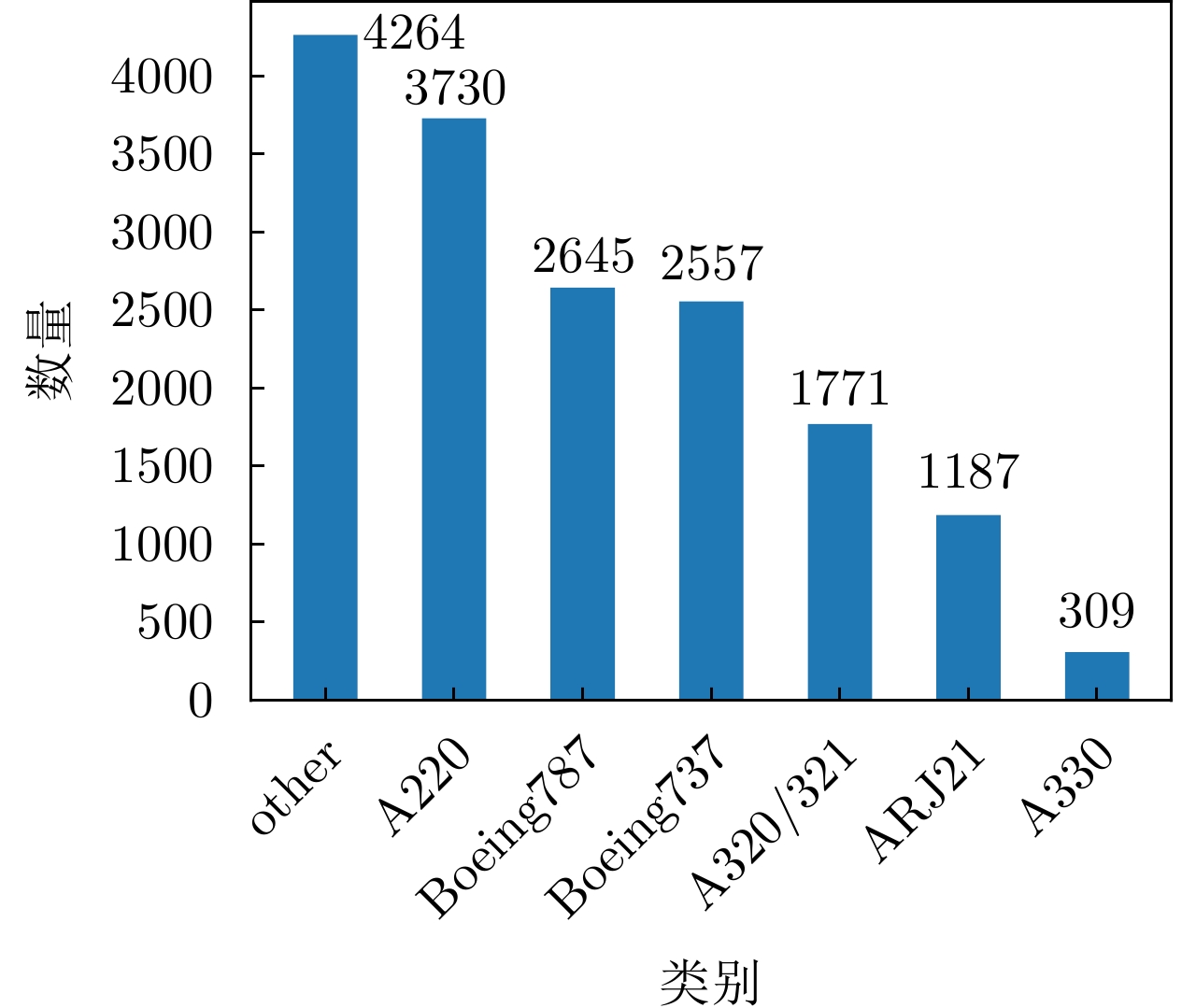
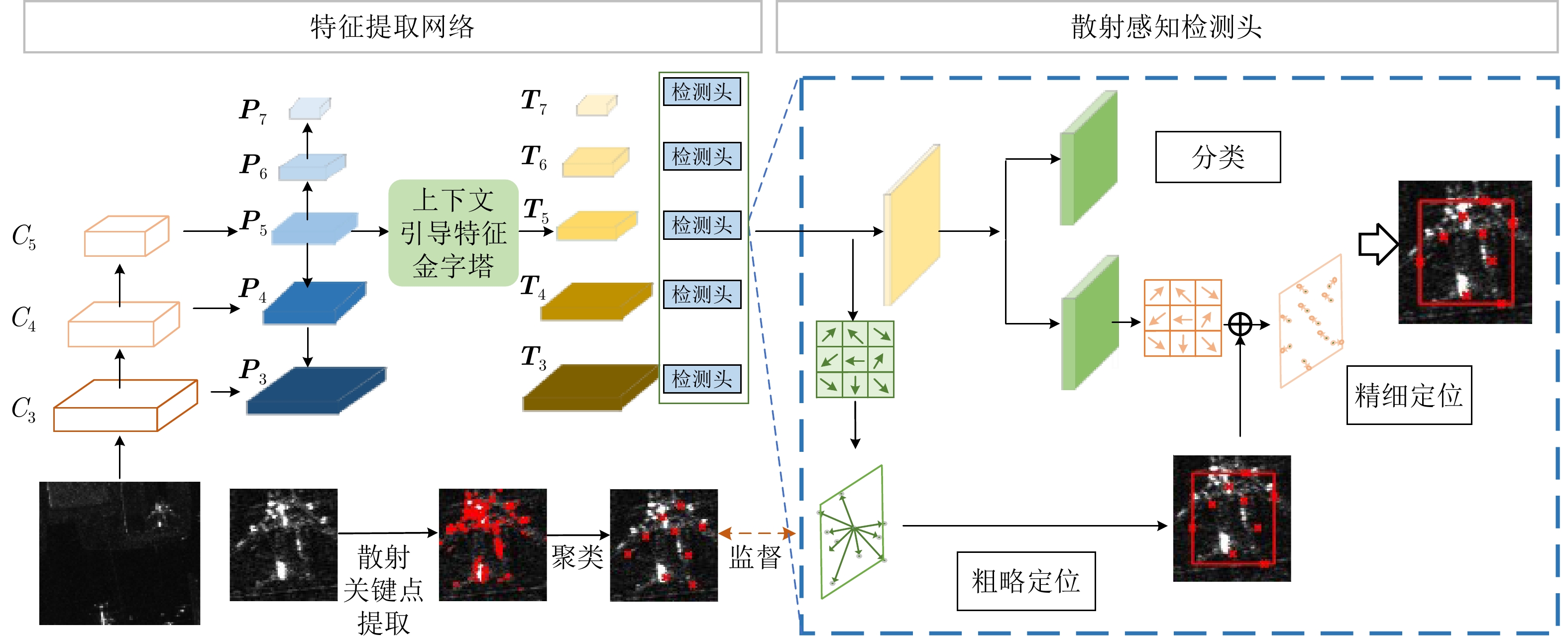
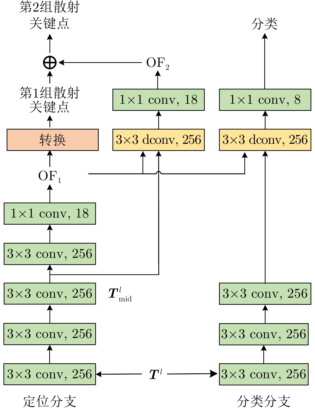
  • This study proposes a Synthetic Aperture Radar (SAR) aircraft detection and recognition method combined with scattering perception to address the problem of target discreteness and false alarms caused by strong background interference in SAR images. The global information is enhanced through a context-guided feature pyramid module, which suppresses strong disturbances in complex images and improves the accuracy of detection and recognition. Additionally, scatter key points are used to locate targets, and a scatter-aware detection module is designed to realize the fine correction of the regression boxes to improve target localization accuracy. This study generates and presents a high-resolution SAR-AIRcraft-1.0 dataset to verify the effectiveness of the proposed method and promote the research on SAR aircraft detection and recognition. The images in this dataset are obtained from the satellite Gaofen-3, which contains 4,368 images and 16,463 aircraft instances, covering seven aircraft categories, namely A220, A320/321, A330, ARJ21, Boeing737, Boeing787, and other. We apply the proposed method and common deep learning algorithms to the constructed dataset. The experimental results demonstrate the excellent effectiveness of our method combined with scattering perception. Furthermore, we establish benchmarks for the performance indicators of the dataset in different tasks such as SAR aircraft detection, recognition, and integrated detection and recognition.


  • Synthetic Aperture Radar (SAR) is an active microwave imaging system capable of all-day, all-weather ground observation. It is unaffected by natural conditions such as lighting, clouds, fog, and weather. SAR has become a crucial information acquisition platform in the field of remote sensing [ 1] . In recent years, with the rapid development of remote sensing imaging technology and the increasing number of in-orbit SAR satellites, the quantity and quality of data obtained by SAR systems have considerably improved, which then promotes SAR’s development and application in relevant fields [ 2] . The vast amount of high-resolution data now available provides a robust foundation for the detailed interpretation of SAR images [ 3, 4] .

    Target detection and recognition are critical steps in the intelligent interpretation of SAR images. As a typical target in SAR images, aircrafts have high observational value because of their abundance and variety [ 5] . Detection and recognition of aircraft in SAR images enable the extraction of information such as aircraft model, type, location, and status. These processes effectively support applications like dynamic monitoring of key areas, situational analysis, and emergency rescue. Therefore, the detection and recognition of aircraft in high-resolution SAR images hold important research value [ 6] .

    In recent years, advances in deep learning theory and technology have led to remarkable progress in target detection and recognition in SAR images using Convolutional Neural Networks (CNNs) [ 7, 8] . For aircraft detection and recognition in SAR images, Zhao et al. [ 9] proposed a multi-branch atrous convolutional feature pyramid method that uses dense connections to reduce redundant information and highlight essential features of aircraft. Ref. [ 10] designed an attention module to refine and integrate low-level texture and high-level semantic features, and the module further improves aircraft detection accuracy. For SAR ship detection and recognition tasks, Refs. [ 11, 12] reduced the dependency on predefined box hyperparameters by directly learning the location of bounding boxes, and they achieved fine-grained ship recognition. Sea vessels often form strong double-bounce reflections with the water surface, and they appear as a complete, highly connected set of strong scatterers in SAR images. In contrast, land-based aircraft are smaller, their features are harder to extract, and their scatterers are more dispersed [ 13, 14] . As such, accurate localization and recognition of land-based aircraft are more challenging.

    In practical scenarios, SAR aircraft detection and recognition present major challenges. First, as shown in Fig. 1(a), aircraft are prone to interference from surrounding backgrounds such as terminals and aprons. Objects with similar scattering properties can be misidentified as aircraft, leading to false alarms and missed detections [ 15] . Second, as shown in Fig. 1(b), aircraft in SAR images appear as a series of discrete, irregularly scattered bright spots with inconsistencies in scattering strength, causing targets to be segmented into multiple discrete parts [ 16] . Consequently, SAR aircraft detection results are incomplete. Third, as shown in Fig. 1(c), the same target exhibits different visual features under various imaging angles, leading to substantial intra-class differences and increased difficulty in aircraft recognition [ 17] .

    Figure  1.  The challenges in SAR aircraft detection and recognition

    To address the issues of severe background interference and dispersed aircraft scatterers in SAR images, this study proposes a Scattering-Aware Network (SA-Net) for detecting and recognizing aircraft targets in complex SAR images. On the one hand, a Context-Guided Feature Pyramid Network (CG-FPN) enhances global information, suppresses strong interference in complex scenes, and improves the discriminative features of the targets. This network thus increases accuracy in detection and recognition. On the other hand, scattering keypoints are utilized for target localization, and a Scattering-Aware detection Head (SA-Head) module is designed to integrate the distribution characteristics of keypoints with the neural network. The correction of the bounding boxes is refined, and the accuracy of target localization is enhanced. To validate the effectiveness of SA-Net, this study constructs SAR-AIRcraft-1.0, a SAR aircraft dataset for large-scale complex scenes. Based on this dataset, a series of detection and recognition comparative experiments are conducted between SA-Net and several commonly used deep neural network models. The experimental results indicate that the SA-Net method achieves an mAP0.5 of 77.7%, showing a notable improvement over the mAP0.5 of other methods. The SA-Net method also demonstrates the excellent performance of the scattering-aware approach. The SAR-AIRcraft-1.0 dataset has been publicly released on the website of the Journal of Radars website ( https://radars.ac.cn/web /data/getData?newsColumnId=f896637b-af23-4209-8bcc-9320fceaba19). This dataset provides a foundation for research on tasks such as SAR aircraft detection, fine-grained recognition, and integrated detection and recognition.

    Most publicly available datasets for SAR detection and recognition tasks focus on ship targets, as shown in Tab. 1. These datasets include MSTAR (The Moving and Stationary Target Acquisition and Recognition) [ 18] , OpenSARShip [ 19] , SSDD (SAR Ship Detection Dataset) [ 20] , SAR-Ship-Dataset [ 21] , AIR-SARShip-1.0 [ 22] , HRSID (High-Resolution SAR Images Dataset) [ 23] , and FUSAR-Ship [ 24] . SAR datasets for aircraft target detection and recognition are relatively limited. Publicly reported datasets include the SAR Aircraft Detection Dataset (SADD) [ 25] and MSAR-1.0 (large-scale Multi-class SAR image target detection dataset-1.0) [ 26] . SADD is an aircraft detection dataset collected from the TerraSAR-X satellite that contains 2,966 image patches. MSAR-1.0 includes four target types: Aircraft, oil tanks, bridges, and ships. These datasets have advanced neural network development for SAR aircraft target detection. However, SADD and MSAR-1.0 only contain positional information for aircraft targets. Both lack fine-grained category annotations for aircraft, which limits further development in SAR aircraft recognition.

    Table  1.  Comparison between the SAR-AIRcraft-1.0 dataset and other SAR object detection datasets
    Dataset Category Instance Image Size Release year Task
    MSTAR 10 5,950 5,950 128×128 1998 Vehicle identification
    OpenSARShip 17 11,346 11,346 256×256 2017 Ship detection and recognition
    SSDD 1 2,456 1,160 190~668 2017 Ship detection
    SAR-Ship-Dataset 1 59,535 43,819 256×256 2019 Ship detection
    AIR-SARShip-1.0 1 461 31 3000× 3000 2019 Ship detection
    HRSID 1 16,951 5,604 800×800 2020 Ship detection and segmentation
    FUSAR-Ship 15 16,144 16,144 512×512 2020 Ship detection and recognition
    SADD 1 7,835 2,966 224×224 2022 Aircraft detection
    MSAR-1.0 4 60,396 28,449 256~2048 2022 Aircraft, oil tanks, bridges, and ships detection
    SAR-AIRcraft-1.0 7 16,463 4,368 800~ 1500 2023 Aircraft detection and identification
     | Show Table
    DownLoad: CSV

    To validate the effectiveness of the SA-Net method and further advance research in SAR aircraft target detection and recognition, this study develops SAR-AIRcraft-1.0, a large-scale SAR aircraft target dataset. The dataset has a resolution of 1 m and includes 4,368 aircraft patches across seven fine-grained aircraft types. SAR-AIRcraft-1.0 is characterized by complex scenes, diverse categories, dense targets, noise interference, varied tasks, and multi-scale properties. The dataset is now publicly accessible on the Journal of Radars website for free use for further studies.

    All images in the SAR-AIRcraft-1.0 dataset are collected by the Gaofen-3 satellite. Single-polarization and a spatial resolution of 1 m are used with the spotlight imaging mode. The dataset primarily includes imagery from three civilian airports: Shanghai Hongqiao Airport, Beijing Capital Airport, and Taiwan Taoyuan Airport. The size of the airport and the number of parked aircraft are considered in the selection of the airports. The dataset contains images in four different sizes—800 × 800, 1000 × 1000, 1200 × 1200, and 1500 × 1500. It comprises a total of 4,368 images and 16,463 aircraft target instances.The aircraft types include A220, A320/321, A330, ARJ21, Boeing737, Boeing787, and other. The latter refers to instances that do not belong to the first six categories). Fig. 2 and Fig. 3 show the instances and quantities of each category. The dataset also has the following features:

    Figure  2.  SAR and optical aircrafts of different categories
    Figure  3.  The quantity of each type of instances

    (1) Complex Scenes: The dataset includes images from multiple time phases of civilian airports. It covers large areas with background features such as terminals, vehicles, and buildings. This coverage increases the complexity of the scenes.

    (2) Rich Categories: Unlike typical SAR aircraft datasets, SAR-AIRcraft-1.0 contains fine-grained category information for aircraft targets. The similar scattering characteristics across different categories make aircraft recognition more challenging.

    (3) Dense Targets: Each image patch includes multiple aircraft targets. As shown in Fig. 1(a), several aircraft are parked near terminals in close proximity. Such proximity creates dense distributions where targets interfere with one another, affecting detection and recognition accuracy.

    (4) Noise Interference: Owing to SAR imaging characteristics, the images contain speckle noise interference, which makes accurate detection and recognition of aircraft targets challenging.

    (5) Varied Tasks: This dataset supports not only detection tasks but also fine-grained recognition because it includes category information. By cropping the aircraft targets, multi-class target patches can be generated, enabling fine-grained recognition. Moreover, with position and category data, SAR-AIRcraft-1.0 supports unified detection-recognition tasks.

    (6) Multi-Scale Characteristics: The aircraft target patches in this dataset vary considerably in size. As shown in Fig. 4, some targets are under 50 × 50 pixels, whereas others exceed 100 × 100 pixels, reflecting a broad multi-scale distribution across targets.

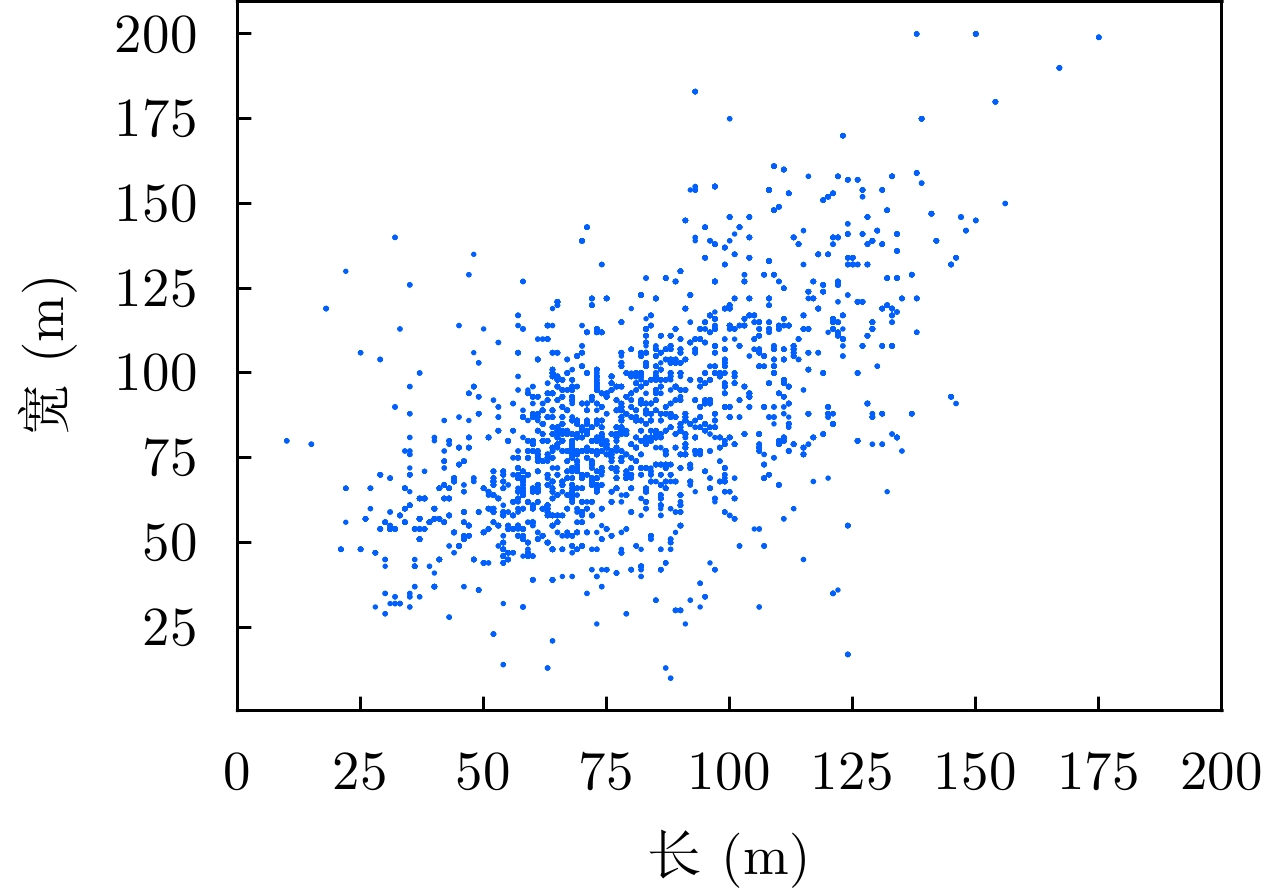
    Figure  4.  The size distribution of aircraft targets

    For instance annotations, all target instances in the SAR-AIRcraft-1.0 dataset are labeled using horizontal bounding boxes. The Pascal VOC format is followed in labeling. Fig. 5(a) shows an example with annotated targets, where orange rectangles represent the bounding boxes. Each box has the target’s category displayed in the top left corner. Each image has a corresponding XML file, as shown in Fig. 5(b), which contains detailed information such as the image size and instance attributes like category and bounding box coordinates.

    Figure  5.  The annotated results in the dataset

    In the XML file, “size” represents the width and height of the image patch, “name” indicates the aircraft category, and “bndbox” provides the coordinate information for each bounding box. With the top-left corner of the image as the origin, “xmin” and “xmax” denote the minimum and maximum X coordinates, whereas “ymin” and “ymax” denote the minimum and maximum Y coordinates, respectively.

    During actual training, the images in the SAR-AIRcraft-1.0 dataset are divided into training, validation, and test sets in a 7:1:2 ratio. The dataset includes multi-temporal images from various airports, encompassing large areas with complex backgrounds. Additionally, because of the imaging mechanism of SAR, images of the same scene taken from different angles exhibit substantial variations, further increasing the complexity of the scenes. Consequently, this dataset presents considerable challenges for detection and recognition tasks.

    To address the issue of strong scattering interference in the background, this study proposes an integrated scattering-aware SAR image aircraft target detection and recognition method. The overall framework, shown in Fig. 6, is based on an anchor-free algorithm structure and consists of two parts: the CG-FPN and SA-Head module.

    Figure  6.  The overall structure of the proposed method

    In the feature extraction network, to mitigate the effect of background interference on target features, this study proposes an improved feature pyramid module to enhance global information and reduce false alarms. The CG-FPN effectively combines contextual information around the target by adaptively adjusting the size of the receptive field, thereby enhancing the saliency features of the target.

    In the target localization phase, this study designs a cascade regression module that combines scattering awareness in a two-stage process to improve the accuracy of the regression boxes. The SA-Head module first detects the scattering keypoints of the target and utilizes their positional information to obtain a rough regression box. Subsequently, the SA-Head module refines the rough regression box to generate more precise detection boxes.

    The overall structure of the CG-FPN is shown in Fig. 7. Suppose the input image is denoted as IRW×H×3, where W and H represent the width and height of the input image, respectively. By downsampling the input image, features from different layers are obtained. Each layer has a size of (W/sl)×(H/sl)×256, where sl=2l represents the downsampling rate of the l(l=3,4,5)th layer, and the channel is set to 256. To obtain the deepest layer features, the features {P3,P4,P5,P6} are resized to a uniform size of P7 and concatenated (concat) along the channel dimension.

    Figure  7.  The framework of context-guided feature pyramid network

    As shown in Fig. 7, CG-FPN applies dilated convolutions with varying dilation rates (rate = 3, 6, 12, 18, 24) on the fused deep features to aggregate multi-scale semantic information through dense connections at each feature level. Each output from the dilated convolution is added to the copied input feature and integrated with the previous layer’s feature before being input into the next layer’s dilated convolution. Finally, the original features are fused with the output features from the dilated convolutions after upsampling. The original features are retained to help the network recall prior information, thus resulting in a feature map that combines shallow detail with deep semantic information.

    Besides integrating features across different layers, CG-FPN seeks to introduce interactive fusion across different channel features. Inspired by the channel attention mechanism of SENet [ 27] , global average pooling [ 28] is first used to compress spatial dimensions and obtain global information. The weights of each feature channel are then adaptively adjusted to reflect inter-channel relationships. Each weight coefficient is multiplied by the corresponding original feature to yield refined features.

    To obtain additional semantic and global information, CG-FPN concatenates the attention feature map A with the feature P7. Based on this, low-resolution features are fused with the corresponding features from the previous layer to generate information-rich features. Finally, a 3 × 3 convolution layer outputs the final feature map TlR(W/sl)×(H/sl)×256. The process is calculated as follows:

    {I7=Concat(Conv1×1(P7)+A)Il=Upsample(Il+1)+Conv1×1(Pl),l=3,4,5,6Tl=Conv3×3(Il),l=3,4,5,6,7 (1)

    This study proposes an SA-Head module that leverages the distribution relationships of scattering points to address discreteness issues. The module consists of localization and classification branches, as shown in Fig. 8, with separate convolution layers for each branch. The output features TlR(W/sl)×(H/sl)×256 from layer l(l=3,4,5,6,7) of the feature extraction network are used as the input features for both branches.

    Figure  8.  The structure of scattering-aware detection head

    In the localization branch, three 3 × 3 convolutional layers are first applied in Tl to obtain intermediate features Tlmid. Subsequently, these features pass through a 3 × 3 convolutional layer with 256 dimensions and a 1 × 1 convolutional layer with 18 dimensions to generate the offset field OF1R(W/sl)×(H/sl)×18. Inspired by DenseBox [ 29] , the first prediction of the scattering keypoints S1 is obtained by the offset from the center point, where their location is given by

    S1={p1i}ni=1={pcenter+Δp1i}ni=1 (2)

    Here, {Δp1i}ni=1 represents the predicted offset from the center point pcenter, taking into account the receptive field size, with n set to 9. p1i=(x1i,y1i) denotes the coordinates of the ith point. After obtaining the predicted scattering keypoints, the coordinates of these points are used to determine the minimum enclosing rectangle B1 in the horizontal and vertical directions. They serve as an initial coarse regression box, thereby identifying the target’s location.

    xmin (3)
    {\boldsymbol{{B}}}_{}^1 = \left( {x_{\min }^1,\;y_{\min }^1,\;x_{\max }^1,\;y_{\max }^1} \right) (4)

    To capture the positional relationships between the aircraft’s scattering points, a supervised learning approach is applied to update the spatial distribution of scattering keypoints through regression. The ground-truth coordinates for these scattering keypoints are obtained as follows [ 17] . First, the Harris corner detector [ 30] is used to identify high-intensity points that reflect structural contours. Second, the k-means algorithm [ 31] clusters these points into 9 clusters, yielding 9 key cluster points with positional offsets relative to the center of the aircraft patch. This process removes redundant points, resulting in a more regular structure. Aircraft patches are cropped based on the ground-truth bounding box (orange box) shown in Fig. 5, and the corresponding XML files contain the bounding box coordinates. Thus, the coordinates of the aircraft patches can be derived from the XML files, and the cluster keypoint coordinates can be calculated using the XML and positional offsets. The nine cluster centers obtained through this method are treated as the ground-truth coordinates of the scattering keypoints. These points reflect the aircraft’s scattering intensity and structural feature distribution, and they provide valuable information for target discrimination.

    During detection, the initial keypoint coordinates of the target are obtained to determine its rough location. However, owing to the scattering mechanism, components within the target that exhibit lower scattering density are often overlooked by the coarse regression box. This oversight results in an imprecise detection box. To address this issue, the SA-Head module employs fine localization to achieve an accurate regression box.

    In fine localization, the first offset group \left\{ {\Delta p_i^1} \right\}_{i = 1}^n and a deformable convolution [ 32] are used to reconstruct the feature {{\boldsymbol{T}}_{{\mathrm{mid}}}} into a new feature map {{\boldsymbol{\tilde T}}_{{\text{mid}}}} \in {R^{\left( {W/{s_l}} \right) \times \left( {H/{s_l}} \right) \times 256}} :

    \begin{split} {\tilde{{\boldsymbol{T}}}}_{\text{mid}}\left(p\right)& ={\Omega }_{3\times \text{3}}\left({{\boldsymbol T}}_{\text{mid}},\;\left\{\Delta {p}_{i}^{1}\right\}\right)\\ & ={\displaystyle \sum _{i=1}^{9}\omega \left(\Delta {p}_{i}^{1}\right)}\cdot {{\boldsymbol{T}}}_{\text{mid}}\left(p+\Delta {p}_{i}^{1}\right) \end{split} (5)

    Here, \omega represents a series of learned weight parameters from the network, and {\Omega _{3 \times {\text{3}}}} indicates the 3 × 3 convolution operation. The calculated offsets may contain some decimal values, so this module draws on bilinear interpolation to produce the continuous feature {{\boldsymbol{T}}_{{\text{mid}}}}\left( {\tilde p} \right){\text{ = }}\displaystyle\sum\nolimits_a {\delta \left( {a,\tilde p} \right)} \cdot {{\boldsymbol{T}}_{{\text{mid}}}}\left( a \right) . In this context, a represents the integral sampling points a = \left( {{x_a},{y_a}} \right) , and \delta \left( {a,\tilde p} \right) is the bilinear interpolation weight between point a and position \tilde p = \left( {{x_{\tilde p}},{y_{\tilde p}}} \right) .

    After obtaining the scattering reconstructed feature {\tilde {\boldsymbol{T}}_{{\mathrm{mid}}}} , this feature is passed through a 1 × 1 convolution layer with an output channel of 18 dimensions to produce a new offset domain {{\mathrm{OF}}_2} . The second set of predicted scattering keypoints {S^2} is obtained as follows:

    {S^2} = \left\{ {\left( {p_i^2} \right)} \right\}_{i = 1}^n = \left\{ {\left( {x_i^2,y_i^2} \right)} \right\}_{i = 1}^n = \left\{ {p_i^1 + \Delta p_i^2} \right\}_{i = 1}^n (6)

    Here, \left\{ {\Delta p_i^2} \right\}_{i = 1}^n represents the predicted offset of the second set of scattering keypoints relative to the first set of keypoints. Using the coordinates of the points, an accurate box position {\boldsymbol{B}}^2 = \left( x_{\min }^2,\;y_{\min }^2, \;x_{\max }^2, \;y_{\max }^2 \right) can be further obtained. Both sets of offsets share the same scale, so the proposed method is unaffected by issues related to the scale parameters of the regression boxes.

    In the classification branch, feature {{\boldsymbol{T}}^l} first passes through three 3 × 3 convolutional layers to extract high-level semantic information about the original features. Similar to the localization branch, it is then processed by a deformable convolution layer with an offset of {{\mathrm{OF}}_1} and a 1 × 1 convolutional layer to optimize and correct the target’s class representation information. This process places greater emphasis on the important scattering components of the SAR aircraft targets. It consequently enhances their relevance and improves the recognition ability of the classification branch. Overall, the SA-Head module integrates the characteristics of the anchor-free framework and utilizes keypoint decoding to obtain the target boxes.

    The overall training loss function can be divided into four parts:

    L = {L_{{{\rm{loc}}} 1}} + {L_{{\rm{loc2}}}} + {L_{{\rm{keypoints}}}} + {L_{{{\rm{cls}}} }} (7)

    where {L_{{\text{loc1}}}} and {L_{{\text{loc2}}}} represent the losses of the first and second predicted boxes compared with the ground truth of the target box. The calculations for {L_{{\mathrm{loc}}}} is as follows:

    {L_{{\text{loc}}}} = \frac{1}{N}\sum\limits_{i = 1}^N {{\text{smoot}}{{\text{h}}_{L1}}\left( {{S_i} - {{\hat S}_i}} \right)} (8)

    Here, N denotes the number of targets, {S_i} and {\hat S_i} represent the predicted box and the ground truth box, respectively, and {{\mathrm{smooth}}_{L1}} is the smoothed {{L}}1 loss function.

    The assumption is that the ground truth coordinates of the target Q scattering keypoints are {\hat S_Q} = \left\{ {{{\hat p}_{iQ}}} \right\}_{i = 1}^n , and the predicted coordinates of the scattering keypoints are S_{Q}=\left\{p_{j Q}\right\}_{j=1}^{m} . Hence, the loss between the predicted coordinates and the ground truth coordinates of the scattering keypoints is calculated using Chamfer loss [ 33] :

    \begin{split} {L_{{\text{keypoints}}}}{\text{ = }}& \frac{1}{N}\sum\limits_{Q = 1}^N \left( \frac{1}{{18}}\sum\limits_{m = 1}^9 \mathop {\min }\limits_n \left\|p_{mQ}^1 - {{\hat p}_{nQ}}\right\|_2\right.\\ & \left.{\text{ + }}\frac{1}{{18}}\sum\limits_{n = 1}^9 {\mathop {\min }\limits_m \left\|p_{mQ}^1 - {{\hat p}_{nQ}}\right\|_2} \right) \end{split} (9)

    Here, n represents the ground truth keypoints of target Q, and m represents the predicted keypoints. As the loss function continues to converge, the model achieves high training accuracy.

    {{\rm{Focalloss}}} \left( {{c_t}} \right) = - {\mu _t}{\left( {1 - {c_t}} \right)^\gamma }\log \left( {{c_t}} \right) (10)

    The classification loss {L_{{\mathrm{cls}}}} uses the focal loss [ 34] function to reduce sample imbalance by adjusting the weights of positive and negative samples. In this function, {\mu _t} = 0.25 and \gamma = 2 are parameters, where {\left( {1 - {c_t}} \right)^\gamma } serves as a modulation factor, and {c_t} is the corresponding classification score.

    In this section, the proposed method is compared with state-of-the-art approaches across various tasks to validate the effectiveness of SA-Net and provide benchmark metrics for the dataset. These tasks include SAR aircraft detection, fine-grained recognition and integrated detection-recognition tasks. Ablation studies are also conducted to further examine the proposed method. Additionally, this section presents a detailed analysis of the experimental outcomes and an outlook on future work.

    ResNet-50 [ 35] , pretrained on the ImageNet dataset, is selected to initialize the model in this study. The batch size is set to 8 for each training iteration, and the model is trained using the stochastic gradient descent algorithm. The initial learning rate is set to 0.001 and decays to 0.0001 after 40 epochs to accelerate convergence. All experiments are conducted on a 16 GB NVIDIA Tesla P100 GPU. The same settings are maintained across all subsequent detection experiments to ensure a fair comparison.

    To quantitatively evaluate the performance of the algorithm, the metrics include precision ( P) and recall ( R), as defined in Eq. (11) and Eq. (12):

    P = \frac{{{{{N}}_{{\text{TP}}}}}}{{{{{N}}_{{\text{TP}}}} + {{{N}}_{{\text{FP}}}}}} (11)
    R = \frac{{{{{N}}_{{\text{TP}}}}}}{{{{{N}}_{{\text{TP}}}}{\text{ + }}{{{N}}_{{\text{FN}}}}}} (12)

    Here, {N_{{\mathrm{TP}}}} represents the number of correctly detected targets. {N_{{\mathrm{FP}}}} refers to the number of false positives where the detection result is positive but the true label is negative (false alarm), and {N_{{\mathrm{FN}}}} denotes the number of false negatives where the detection result is negative but the true label is positive (missed detection). The {\mathrm{F1 }}-score is used to provide a comprehensive evaluation of the algorithm’s performance, defined as follows:

    {\text{F1}} = \frac{{2 \times P \times R}}{{P + R}} (13)

    In addition, this study utilizes the Precision-Recall Curve (PRC) and Average Precision (AP). The PRC can be plotted By sorting predictions in descending order of confidence and calculating precision-recall pairs at different steps. AP reflects the shape of the PRC and provides a comprehensive evaluation of the algorithm’s performance. AP is defined as the mean of the highest precision values over a set of recall rates S = {0, 0.01, 0.02, ···, 1}, with the specific calculation given by

    {\text{AP}} = \frac{1}{{101}}\sum\limits_{R \in S} {\tilde P\left( R \right)} (14)

    Here, \tilde P\left( R \right) = \max _{R':R' \ge R} P\left( {R'} \right) is the precision corresponding to each recall R, and P\left( {R'} \right) is the precision corresponding to recall R'. After calculating the AP for each category, the mean Average Precision (mAP) is obtained as the average of AP values across all categories. Typically, AP is calculated with an Intersection-over-Union (IoU) threshold of 0.5, denoted as AP 0.5.

    Target detection is a fundamental task in SAR imaging. This study utilizes the SAR-AIRcraft-1.0 dataset to train and test several widely used benchmark detection methods, including Faster R-CNN [ 36] and Cascade R-CNN [ 37] . Both are two-stage CNNs. Recently, anchor-free, single-stage detection methods have been designed to greatly reduce sensitivity to anchor-related parameters. Consequently, the classic anchor-free method RepPoints [ 38] and an SAR-specific target detection method, namely SKG-Net [ 1] , are compared.

    In terms of data utilization, all aircraft targets are treated as positive samples, and the background as negative samples. All aircraft targets are categorized into a single class. Tab. 2 presents the accuracy, recall, F1-score, AP 0.5, and AP 0.75 metrics for aircraft targets across different detectors. The results indicate that SA-Net achieves the highest accuracy across different thresholds, demonstrating the effectiveness of the proposed method.

    Table  2.  Detection results of different methods (%)
    Detection methods P R F1 AP 0.5 AP 0.75
    Faster R-CNN 77.6 78.1 77.8 71.6 53.6
    Cascade R-CNN 89.0 79.5 84.0 77.8 59.1
    RepPoints 62.7 88.7 81.2 80.3 52.9
    SKG-Net 57.6 88.8 69.9 79.8 51.0
    SA-Net 87.5 82.2 84.8 80.4 61.4
     | Show Table
    DownLoad: CSV

    In the detection methods discussed above, most anchor boxes are redundant because of the sparse distribution of SAR aircraft targets. Anchor-free detection algorithms achieve better results on AP 0.5, with RepPoints and SKG-Net reaching 80.3% and 79.8%, respectively. This improvement may be due to anchor-free methods reducing background clutter within bounding boxes, thereby clarifying the semantic information of the targets. However, RepPoints and SKG-Net produce more false positives (false alarms) compared with anchor-based methods, reducing detection accuracy.

    Among two-stage detection methods, the cascade structure of Cascade R-CNN further improves AP and various metrics compared with Faster R-CNN. Fig. 9 shows visual comparisons of the test results between the proposed method and other advanced methods. The figure illustrates that Faster R-CNN, RepPoints, and Cascade R-CNN all exhibit false positives (yellow) and false negatives (blue boxes). By contrast, SA-Net effectively reduces these false positives and negatives, validating its superior detection performance.

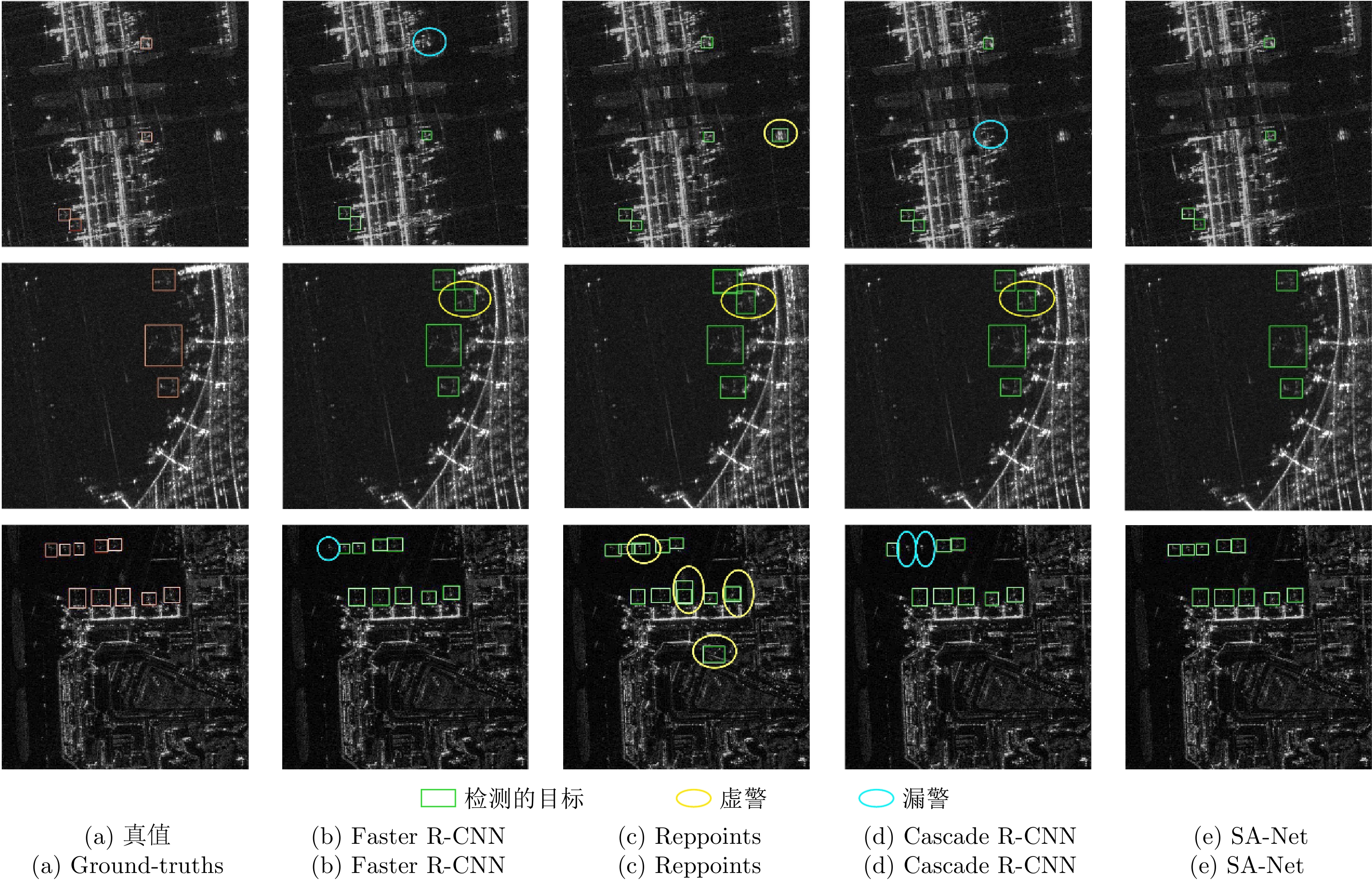
    Figure  9.  The visualization results

    In this study, instance targets are cropped according to the annotation boxes in the SAR-AIRcraft-1.0 dataset, resulting in a series of instance samples. The specific quantities are shown in Tab. 3. For the fine-grained recognition experiments, seven distinct aircraft labels are selected: A330, A320/321, A220, ARJ21, Boeing 737, Boeing 787, and other.

    Table  3.  The number of instance targets of different categories
    Category Training set number Test set number Total
    A330 278 31 309
    A320/321 1719 52 1771
    A220 3270 460 3730
    ARJ21 825 362 1187
    Boeing737 2007 550 2557
    Boeing787 2191 454 2645
    other 3223 1041 4264
    Total 13513 2950 16463
     | Show Table
    DownLoad: CSV

    This study uses recognition accuracy as the evaluation metric to quantify the performance of the fine-grained recognition task. The corresponding calculation is given by Eq. (15):

    {\text{Acc}} = \frac{{\displaystyle\sum\nolimits_i {{N_{{C_i}}}} }}{{{N_{{\text{all}}}}}} (15)

    where {N_{{C_i}}} represents the number of correctly identified samples for class {C_i} , and N represents the total number of samples.

    This study conducts experimental comparison using ResNet-50, ResNet-101, ResNeXt-50, ResNeXt-101 [ 39] , and Swin Transformer [ 40] on the SAR-AIRcraft-1.0 dataset. Fifty percent of the data from the training set are selected for model training. The results of the fine-grained recognition are presented in Tab. 4, which shows that ResNet-101 outperforms ResNet-50. The ResNeXt series of models achieve excellent performance in terms of top-1 recognition accuracy. The Swin Transformer not only exhibits the highest performance in top-3 accuracy but also achieves the best recognition capability in most categories. This outcome demonstrates its outstanding feature learning ability.

    Table  4.  Fine-grained recognition results (%)
    Methods Acc (top-1/top-3) A330 A320/321 A220 ARJ21 Boeing737 Boeing787 Other
    ResNet-50 75.59/89.19 74.19 90.38 78.04 73.76 61.64 78.63 80.50
    ResNet-101 78.58/90.37 93.55 98.08 76.96 73.76 71.82 74.67 84.82
    ResNeXt-50 80.61/89.46 83.87 94.23 78.91 74.86 73.27 83.04 85.40
    ResNeXt-101 82.20/91.83 87.10 100 80.87 79.83 71.09 83.92 87.70
    Swin Trarsformer 81.29/ 92.51 77.42 100 80.87 74.59 73.82 86.12 84.82
     | Show Table
    DownLoad: CSV

    To further quantitatively assess the model’s performance and display additional details of the recognition results, this study presents a confusion matrix of the algorithm models to show the performance of different network architectures. As illustrated in Fig. 10, the probabilities along the diagonal represent the recognition accuracy for each category. Among them, the identification of aircraft targets such as A330, ARJ21, and Boeing 737 proves to be challenging, reflected by their relatively low recognition accuracy. The images of Boeing 737 and Boeing 787 are quite similar, resulting in confusion in the recognition results. This situation highlights the challenges posed by the SAR-AIRcraft-1.0 dataset.

    Figure  10.  The confusion matrices for the methods

    This study selects four distinct methods for comparative experiments on integrated detection and recognition to validate the performance of different deep learning algorithms. These four methods are Faster R-CNN, Cascade R-CNN, Reppoints, and SKG-Net, which encompass anchor-based and anchor-free approaches.

    During the experiments, different categories of aircraft are treated as separate classes. No data augmentation techniques are employed to maintain the original characteristics of the data. The detection performance of each algorithm is displayed in Tab. 5. For the Faster R-CNN method, the mAP 0.5 for various categories is 76.1%, and the mAP 0.75 is 62.2%. Thus, the SAR-AIRcraft-1.0 dataset presents certain detection challenges. First, different categories of SAR aircraft targets share similar structures and sizes, so distinguishing between target classes is difficult. Furthermore, owing to the scattering characteristics of SAR images and variations in imaging conditions, targets of the same category may yield different imaging results. The recognition process becomes increasingly complicated.

    Table  5.  The performance of the algorithms based on deep learning (IoU=0.5)
    Category Faster
    R-CNN
    Cascade
    R-CNN
    Reppoints SKG-Net SA-Net
    A330 85.0 87.4 89.8 79.3 88.6
    A320/321 97.2 97.5 97.9 78.2 94.3
    A220 78.5 74.0 71.4 66.4 80.3
    ARJ21 74.0 78.0 73.0 65.0 78.6
    Boeing737 55.1 54.5 55.7 65.1 59.7
    Boeing787 72.9 68.3 51.8 69.6 70.8
    other 70.1 69.1 68.4 71.4 71.3
    mAP 76.1 75.7 72.6 70.7 77.7
     | Show Table
    DownLoad: CSV

    Additionally, this study selects a more stringent metric, AP at the IoU threshold of 0.75 (AP 0.75), to evaluate the model, as shown in Tab. 6. Given the integration of global contextual features and scattering information, the proposed SA-Net achieves an mAP 0.75 of 62.8%. However, the detection accuracy varies among different categories. For instance, compared with other categories, the A320/321 demonstrates the best performance in AP 0.5 and AP 0.75 across various algorithms. This outcome is primarily because the A320/321 has a distinctive size, with a fuselage length of over 40 m, making it easy to differentiate. For ARJ21 and A220, their relatively small size and insufficient detail features lower detection accuracy.

    Table  6.  The performance of the algorithms based on deep learning (IoU=0.75)
    Category Faster
    R-CNN
    Cascade
    R-CNN
    Reppoints SKG-Net SA-Net
    A330 85.0 87.4 66.4 66.4 88.6
    A320/321 87.7 73.9 84.9 49.6 86.6
    A220 58.7 49.1 49.4 29.8 55.0
    ARJ21 55.2 59.0 50.9 37.7 59.7
    Boeing737 42.8 39.1 36.6 48.7 41.8
    Boeing787 60.5 57.6 41.8 51.6 60.4
    other 45.4 46.1 43.1 41.1 47.7
    mAP 62.2 58.9 53.3 46.4 62.8
     | Show Table
    DownLoad: CSV

    To intuitively compare various methods, this study plots the F1 curves of different methods at various thresholds, as shown in Fig. 11. The figure depicts that SA-Net consistently achieves the highest F1 score across different confidence levels compared with other advanced methods. This finding indicates that the proposed method exhibits good robustness, achieving a strong balance between detection rate and recall rate.

    Figure  11.  F1 curves of different advanced methods

    This study combines the FCOS [ 41] with deformable convolution as the baseline network. Ablation experiments are conducted on the SAR-AIRcraft-1.0 dataset with different modules, and the results are shown in Tab. 7. The proposed modules contribute to varying degrees of improvement in detection performance. Compared with the baseline, the CG-FPN module improves the AP 0.5 metric by 0.8%. The AP 0.5 and AP 0.75 of the SA-Net are 0.8% and 0.7% higher than those of the baseline, respectively, achieving more accurate localization of the targets.

    Table  7.  Influence of each component in the proposed method (%)
    Methods P R F1 AP 0.5 AP 0.75
    Baseline 88.1 81.2 84.5 79.6 60.7
    Baseline+SA-Head 88.2 82.1 85.0 80.3 60.8
    Baseline+CG-FPN 88.6 81.9 85.1 80.4 60.4
    SA-Net 87.5 82.2 84.8 80.4 61.4
     | Show Table
    DownLoad: CSV

    To visually compare different modules, Fig. 12 and Fig. 13 present the corresponding F1 curves and PR curves. Fig. 12 depicts that SA-Net achieves optimal results in AP 0.5 and AP 0.75, demonstrating the best performance in the high-confidence range of the F1 curve. This study introduces the SA-Head module to achieve more accurate localization of detection boxes. Fig. 13 demonstrates that the PR curve with the SA-Head module (orange curve) shows substantial improvement in AP 0.5 and AP 0.75 compared with the baseline (blue curve), indicating that the SA-Head module can enhance the network’s detection performance.

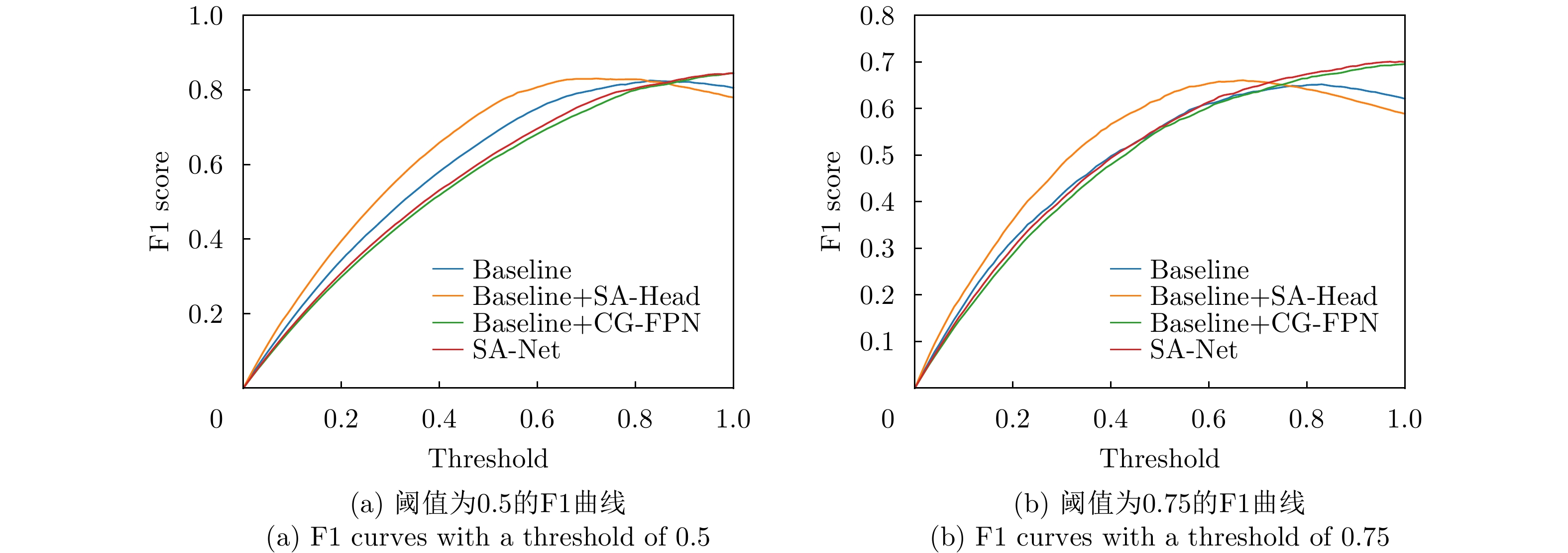
    Figure  12.  F1 curves of different improvements in the proposed method
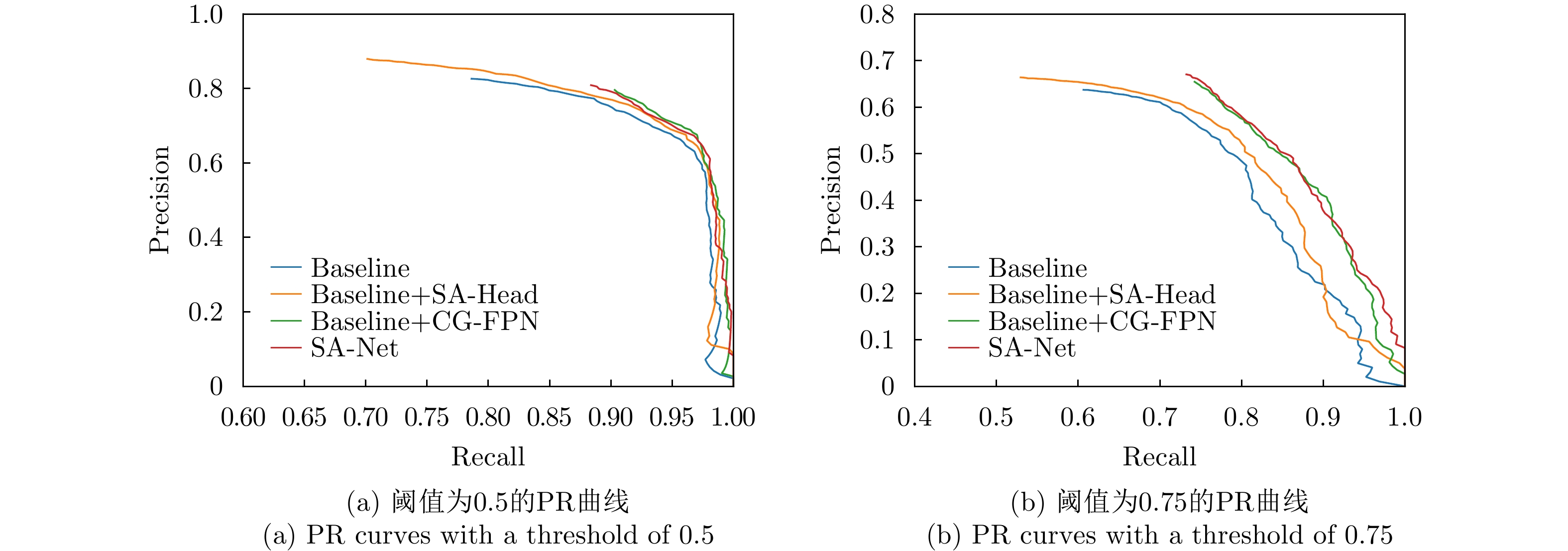
    Figure  13.  PR curves of different improvements in the proposed method

    Additionally, this study introduces CG-FPN to strengthen global features and suppress scattering interference in the background. Fig. 14 displays detection results and visualization effects, where green rectangles and yellow circles represent detected targets and false alarms, respectively. As shown in Fig. 14(a), the baseline produces false alarms because of similar buildings in the background. To address this issue, CG-FPN enhances the contextual connections of features by assigning different weights to channel layers. The feature map from the last layer of the classification branch is visualized for a direct comparison. Fig. 14(c) and Fig. 14(d) show that after adding this module, the aircraft targets receive more attention. The experimental results prove that CG-FPN effectively enhances the saliency of targets and reduces false alarms in complex backgrounds.

    Figure  14.  Detection results and visualization

    This study conducts a series of experiments using different detection algorithms on the SAR-AIRcraft-1.0 dataset. The results demonstrate that the proposed SA-Net method exhibits superior performance. Detection results are shown in Fig. 15. Green rectangles, yellow circles, blue circles, and red circles represent detection results, false alarms, missed detections, and incorrectly identified targets, respectively. Most targets in the SA-Net method are accurately detected, but false alarms and missed detections still exist. The false alarms are primarily due to scattering representations similar to aircraft near complex backgrounds, such as terminals. Additionally, the variability in scattering conditions leads to weaker scattering of certain aircraft components. This scattering thus affects the semantic integrity of target features and results in missed detections.

    Figure  15.  Detection results of SA-Net

    In addition to these issues, Fig. 15 shows incorrectly identified instances marked with red circles. Owing to the small size of the targets and the lack of semantic features, some aircraft are misidentified as other categories. The absence of prior information, such as aircraft length, makes correctly distinguishing between different categories more challenging. Overall, detecting and identifying targets in the SAR-AIRcraft-1.0 dataset is a difficult task. The current algorithms still exhibit unsatisfactory performance, indicating further room for improvement. In future work, incorporating SAR imaging mechanisms and scattering features into deep CNNs may further enhance the detection and identification performance of the SAR-AIRcraft-1.0 dataset.

    This study proposes a SAR aircraft detection and recognition method that incorporates scattering perception. It utilizes a CG-FPN to enhance global information and suppress strong interference in complex scenes, thereby achieving effective feature fusion and reducing false alarms and missed detections. The method also employs scattering keypoints to refine and correct detection boxes, improving localization accuracy. To validate the effectiveness of the proposed method, this study publicly releases a high-resolution SAR-AIRcraft-1.0 dataset. This dataset contains various categories of aircraft targets. It is characterized by complex scenes, diverse categories, dense targets, noise interference, diverse tasks, and multi-scale features. The dataset provides rich data for model training and facilitating research in SAR aircraft detection and recognition. Experiments conducted on the SAR-AIRcraft-1.0 dataset demonstrate the effectiveness of the proposed approach compared with other deep learning algorithms. In future work, integrating scattering feature information into deep CNNs can further enhance detection and recognition performance.

    SAR-AIRcraft-1.0: The high-resolution SAR aircraft detection and recognition dataset is released on the official website of the Journal of Radars, and the data and usage instructions are uploaded to the journal’s website on the “SAR-AIRcraft-1.0: High-Resolution SAR Aircraft Detection and Recognition Dataset” page (see Fig. 1). The URL is https://radars.ac.cn/web/data/getData?newsColumnId=f896637b-af23-4209-8bcc-9320fceaba19.

    1.  Release webpage of SAR-AIRcraft-1.0: High-resolution SAR aircraft detection and recognition dataset
  • [1]
    FU Kun, FU Jiamei, WANG Zhirui, et al. Scattering-keypoint-guided network for oriented ship detection in high-resolution and large-scale SAR images[J]. IEEE Journal of Selected Topics in Applied Earth Observations and Remote Sensing, 2021, 14: 11162–11178. doi: 10.1109/JSTARS.2021.3109469.
    [2]
    GUO Qian, WANG Haipeng, and XU Feng. Scattering enhanced attention pyramid network for aircraft detection in SAR images[J]. IEEE Transactions on Geoscience and Remote Sensing, 2021, 59(9): 7570–7587. doi: 10.1109/TGRS.2020.3027762.
    [3]
    SHAHZAD M, MAURER M, FRAUNDORFER F, et al. Buildings detection in VHR SAR images using fully convolution neural networks[J]. IEEE Transactions on Geoscience and Remote Sensing, 2019, 57(2): 1100–1116. doi: 10.1109/TGRS.2018.2864716.
    [4]
    ZHANG Zhimian, WANG Haipeng, XU Feng, et al. Complex-valued convolutional neural network and its application in polarimetric SAR image classification[J]. IEEE Transactions on Geoscience and Remote Sensing, 2017, 55(12): 7177–7188. doi: 10.1109/TGRS.2017.2743222.
    [5]
    FU Kun, DOU Fangzheng, LI Hengchao, et al. Aircraft recognition in SAR images based on scattering structure feature and template matching[J]. IEEE Journal of Selected Topics in Applied Earth Observations and Remote Sensing, 2018, 11(11): 4206–4217. doi: 10.1109/JSTARS.2018.2872018.
    [6]
    DU Lan, DAI Hui, WANG Yan, et al. Target discrimination based on weakly supervised learning for high-resolution SAR images in complex scenes[J]. IEEE Transactions on Geoscience and Remote Sensing, 2020, 58(1): 461–472. doi: 10.1109/TGRS.2019.2937175.
    [7]
    CUI Zongyong, LI Qi, CAO Zongjie, et al. Dense attention pyramid networks for multi-scale ship detection in SAR images[J]. IEEE Transactions on Geoscience and Remote Sensing, 2019, 11: 8983–8997. doi: 10.1109/TGRS.2019.2923988.
    [8]
    ZHANG Jinsong, XING Mengdao, and XIE Yiyuan. FEC: A feature fusion framework for SAR target recognition based on electromagnetic scattering features and deep CNN features[J]. IEEE Transactions on Geoscience and Remote Sensing, 2021, 59(3): 2174–2187. doi: 10.1109/TGRS.2020.3003264.
    [9]
    ZHAO Yan, ZHAO Lingjun, LI Chuyin, et al. Pyramid attention dilated network for aircraft detection in SAR images[J]. IEEE Geoscience and Remote Sensing Letters, 2021, 18(4): 662–666. doi: 10.1109/LGRS.2020.2981255.
    [10]
    ZHAO Yan, ZHAO Lingjun, LIU Zhong, et al. Attentional feature refinement and alignment network for aircraft detection in SAR imagery[J]. IEEE Transactions on Geoscience and Remote Sensing, 2022, 60: 5220616. doi: 10.1109/TGRS.2021.3139994.
    [11]
    FU Jiamei, SUN Xian, WANG Zhirui, et al. An anchor-free method based on feature balancing and refinement network for multiscale ship detection in SAR images[J]. IEEE Transactions on Geoscience and Remote Sensing, 2021, 59(2): 1331–1344. doi: 10.1109/TGRS.2020.3005151.
    [12]
    SUN Yuanrui, WANG Zhirui, SUN Xian, et al. SPAN: Strong scattering point aware network for ship detection and classification in large-scale SAR imagery[J]. IEEE Journal of Selected Topics in Applied Earth Observations and Remote Sensing, 2022, 15: 1188–1204. doi: 10.1109/JSTARS.2022.3142025.
    [13]
    郭倩, 王海鹏, 徐丰. SAR图像飞机目标检测识别进展[J]. 雷达学报, 2020, 9(3): 497–513. doi: 10.12000/JR20020.

    GUO Qian, WANG Haipeng, and XU Feng. Research progress on aircraft detection and recognition in SAR imagery[J]. Journal of Radars, 2020, 9(3): 497–513. doi: 10.12000/JR20020.
    [14]
    吕艺璇, 王智睿, 王佩瑾, 等. 基于散射信息和元学习的SAR图像飞机目标识别[J]. 雷达学报, 2022, 11(4): 652–665. doi: 10.12000/JR22044.

    LYU Yixuan, WANG Zhirui, WANG Peijin, et al. Scattering information and meta-learning based SAR images interpretation for aircraft target recognition[J]. Journal of Radars, 2022, 11(4): 652–665. doi: 10.12000/JR22044.
    [15]
    KANG Yuzhuo, WANG Zhirui, FU Jiamei, et al. SFR-Net: Scattering feature relation network for aircraft detection in complex SAR images[J]. IEEE Transactions on Geoscience and Remote Sensing, 2022, 60: 5218317. doi: 10.1109/TGRS.2021.3130899.
    [16]
    CHEN Jiehong, ZHANG Bo, and WANG Chao. Backscattering feature analysis and recognition of civilian aircraft in TerraSAR-X images[J]. IEEE Geoscience and Remote Sensing Letters, 2015, 12(4): 796–800. doi: 10.1109/LGRS.2014.2362845.
    [17]
    SUN Xian, LV Yixuan, WANG Zhirui, et al. SCAN: Scattering characteristics analysis network for few-shot aircraft classification in high-resolution SAR images[J]. IEEE Transactions on Geoscience and Remote Sensing, 2022, 60: 5226517. doi: 10.1109/TGRS.2022.3166174.
    [18]
    KEYDEL E R, LEE S W, and MOORE J T. MSTAR extended operating conditions: A tutorial[C]. The SPIE 2757, Algorithms for Synthetic Aperture Radar Imagery III, Orlando, USA, 1996: 228–242.
    [19]
    HUANG Lanqing, LIU Bin, LI Boying, et al. OpenSARShip: A dataset dedicated to Sentinel-1 ship interpretation[J]. IEEE Journal of Selected Topics in Applied Earth Observations and Remote Sensing, 2018, 11(1): 195–208. doi: 10.1109/JSTARS.2017.2755672.
    [20]
    LI Jianwei, QU Changwen, and SHAO Jiaqi. Ship detection in SAR images based on an improved faster R-CNN[C]. 2017 SAR in Big Data Era: Models, Methods and Applications (BIGSARDATA), Beijing, China, 2017: 1–6.
    [21]
    WANG Yuanyuan, WANG Chao, ZHANG Hong, et al. A SAR dataset of ship detection for deep learning under complex backgrounds[J]. Remote Sensing, 2019, 11(7): 765. doi: 10.3390/rs11070765.
    [22]
    孙显, 王智睿, 孙元睿, 等. AIR-SARShip-1.0: 高分辨率SAR舰船检测数据集[J]. 雷达学报, 2019, 8(6): 852–862. doi: 10.12000/JR19097.

    SUN Xian, WANG Zhirui, SUN Yuanrui, et al. AIR-SARShip-1.0: High-resolution SAR ship detection dataset[J]. Journal of Radars, 2019, 8(6): 852–862. doi: 10.12000/JR19097.
    [23]
    WEI Shunjun, ZENG Xiangfeng, QU Qizhe, et al. HRSID: A high-resolution SAR images dataset for ship detection and instance segmentation[J]. IEEE Access, 2020, 8: 120234–120254. doi: 10.1109/ACCESS.2020.3005861.
    [24]
    HOU Xiyue, AO Wei, SONG Qian, et al. FUSAR-Ship: Building a high-resolution SAR-AIS matchup dataset of Gaofen-3 for ship detection and recognition[J]. Science China Information Sciences, 2020, 63(4): 140303. doi: 10.1007/s11432-019-2772-5.
    [25]
    ZHANG Peng, XU Hao, TIAN Tian, et al. SEFEPNet: Scale expansion and feature enhancement pyramid network for SAR aircraft detection with small sample dataset[J]. IEEE Journal of Selected Topics in Applied Earth Observations and Remote Sensing, 2022, 15: 3365–3375. doi: 10.1109/JSTARS.2022.3169339.
    [26]
    陈杰, 黄志祥, 夏润繁, 等. 大规模多类SAR目标检测数据集-1.0[J/OL]. 雷达学报. https://radars.ac.cn/web/data/getData?dataType=MSAR, 2022.

    CHEN Jie, HUANG Zhixiang, XIA Runfan, et al. Large-scale multi-class SAR image target detection dataset-1.0[J/OL]. Journal of Radars. https://radars.ac.cn/web/data/getData?dataType=MSAR, 2022.
    [27]
    HU Jie, SHEN Li, and SUN Gang. Squeeze-and-excitation networks[C]. IEEE/CVF Conference on Computer Vision and Pattern Recognition, Salt Lake City, USA, 2018: 7132–7141.
    [28]
    SUN Yuanrui, SUN Xian, WANG Zhirui, et al. Oriented ship detection based on strong scattering points network in large-scale SAR images[J]. IEEE Transactions on Geoscience and Remote Sensing, 2021, 60: 5218018. doi: 10.1109/TGRS.2021.3130117.
    [29]
    HUANG Lichao, YANG Yi, DENG Yafeng, et al. DenseBox: Unifying landmark localization with end to end object detection[J]. arXiv preprint arXiv: 1509.04874, 2015.
    [30]
    MIKOLAJCZYK K and SCHMID C. Scale & affine invariant interest point detectors[J]. International Journal of Computer Vision, 2004, 60(1): 63–86. doi: 10.1023/B:VISI.0000027790.02288.f2.
    [31]
    OLUKANMI P O, NELWAMONDO F, and MARWALA T. K-means-MIND: An efficient alternative to repetitive k-means runs[C]. 2020 7th International Conference on Soft Computing & Machine Intelligence (ISCMI), Stockholm, Sweden, 2020: 172–176.
    [32]
    DAI Jifeng, QI Haozhi, XIONG Yuwen, et al. Deformable convolutional networks[C]. 2017 IEEE International Conference on Computer Vision, Venice, Italy, 2017: 764–773.
    [33]
    FAN Haoqiang, SU Hao, and GUIBAS L. A point set generation network for 3d object reconstruction from a single image[C]. 2017 IEEE Conference on Computer Vision and Pattern Recognition, Honolulu, USA, 2017: 2463–2471.
    [34]
    LIN T Y, GOYAL P, GIRSHICK R, et al. Focal loss for dense object detection[C]. 2017 IEEE International Conference on Computer Vision, Venice, Italy, 2017: 2999–3007.
    [35]
    HE Kaiming, ZHANG Xiangyu, REN Shaoqing, et al. Deep residual learning for image recognition[C]. 2016 IEEE Conference on Computer Vision and Pattern Recognition, Las Vegas, USA, 2016: 770–778.
    [36]
    GIRSHICK R. Fast R-CNN[C]. 2015 IEEE International Conference on Computer Vision, Santiago, Chile, 2015: 1440–1448.
    [37]
    CAI Zhaowei and VASCONCELOS N. Cascade R-CNN: Delving into high quality object detection[C]. 2018 IEEE/CVF Conference on Computer Vision and Pattern Recognition, Salt Lake City, USA, 2018: 6154–6162.
    [38]
    YANG Ze, LIU Shaohui, HU Han, et al. RepPoints: Point set representation for object detection[C]. 2019 IEEE/CVF International Conference on Computer Vision, Seoul, Korea, 2019: 9656–9665.
    [39]
    XIE Saining, GIRSHICK R, DOLLÁR P, et al. Aggregated residual transformations for deep neural networks[C]. 2017 IEEE Conference on Computer Vision and Pattern Recognition, Honolulu, USA, 2017: 5987–5995.
    [40]
    LIU Ze, LIN Yutong, CAO Yue, et al. Swin transformer: Hierarchical vision transformer using shifted windows[C]. 2021 IEEE/CVF International Conference on Computer Vision, Montreal, Canada, 2021: 9992–10002.
    [41]
    TIAN Zhi, SHEN Chunhua, CHEN Hao, et al. FCOS: Fully convolutional one-stage object detection[C]. 2019 IEEE/CVF International Conference on Computer Vision, Seoul, Korea, 2019: 9626–9635.
  • Relative Articles

    [1]CHEN Xiaolong, RAO Guilin, GUAN Jian, WANG Jinhao, WANG Hongyong, ZHANG Caisheng, YI Jianxin, WAN Xianrong, RAO Yunhua. Passive Radar Low Slow Small Detection Dataset (LSS-PR-1.0) and Multi-domain Feature Extraction and Analysis Methods[J]. Journal of Radars. doi: 10.12000/JR24145
    [2]CHEN Xiaolong, Yuan Wang, Du Xiaolin, Yu Gang, He Xiaoyang, Guan Jian, Wang Xinghai. Multiband FMCW Radar LSS-target Detection Dataset (LSS-FMCWR-1.0) and High-resolution Micromotion Feature Extraction Method[J]. Journal of Radars, 2024, 13(3): 539-553. doi: 10.12000/JR23142
    [3]WANG Xiang, WANG Yumiao, CHEN Xingyu, ZANG Chuanfei, CUI Guolong. Deep Learning-based Marine Target Detection Method with Multiple Feature Fusion[J]. Journal of Radars, 2024, 13(3): 554-564. doi: 10.12000/JR23105
    [4]LUO Ru, ZHAO Lingjun, HE Qishan, JI Kefeng, KUANG Gangyao. Intelligent Technology for Aircraft Detection and Recognition through SAR Imagery: Advancements and Prospects[J]. Journal of Radars, 2024, 13(2): 307-330. doi: 10.12000/JR23056
    [5]CHEN Xiang, WANG Liandong, XU Xiong, SHEN Xujian, FENG Yuntian. A Review of Radio Frequency Fingerprinting Methods Based on Raw I/Q and Deep Learning[J]. Journal of Radars, 2023, 12(1): 214-234. doi: 10.12000/JR22140
    [6]TIAN Ye, DING Chibiao, ZHANG Fubo, SHI Min’an. SAR Building Area Layover Detection Based on Deep Learning[J]. Journal of Radars, 2023, 12(2): 441-455. doi: 10.12000/JR23033
    [7]DU Lan, CHEN Xiaoyang, SHI Yu, XUE Shikun, XIE Meng. MMRGait-1.0: A Radar Time-frequency Spectrogram Dataset for Gait Recognition under Multi-view and Multi-wearing Conditions[J]. Journal of Radars, 2023, 12(4): 892-905. doi: 10.12000/JR22227
    [8]DING Zihang, XIE Junwei, WANG Bo. Missing Covariance Matrix Recovery with the FDA-MIMO Radar Using Deep Learning Method[J]. Journal of Radars, 2023, 12(5): 1112-1124. doi: 10.12000/JR23002
    [9]HE Mi, PING Qinwen, DAI Ran. Fall Detection Based on Deep Learning Fusing Ultrawideband Radar Spectrograms[J]. Journal of Radars, 2023, 12(2): 343-355. doi: 10.12000/JR22169
    [10]CHEN Siwei, CUI Xingchao, LI Mingdian, TAO Chensong, LI Haoliang. SAR Image Active Jamming Type Recognition Based on Deep CNN Model[J]. Journal of Radars, 2022, 11(5): 897-908. doi: 10.12000/JR22143
    [11]HUANG Zhongling, YAO Xiwen, HAN Junwei. Progress and Perspective on Physically Explainable Deep Learning for Synthetic Aperture Radar Image Interpretation(in English)[J]. Journal of Radars, 2022, 11(1): 107-125. doi: 10.12000/JR21165
    [12]XU Congan, SU Hang, LI Jianwei, LIU Yu, YAO Libo, GAO Long, YAN Wenjun, WANG Taoyang. RSDD-SAR: Rotated Ship Detection Dataset in SAR Images[J]. Journal of Radars, 2022, 11(4): 581-599. doi: 10.12000/JR22007
    [13]MA Lin, PAN Zongxu, HUANG Zhongling, HAN Bing, HU Yuxin, ZHOU Xiao, LEI Bin. Multichannel False-target Discrimination in SAR Images Based on Sub-aperture and Full-aperture Feature Learning[J]. Journal of Radars, 2021, 10(1): 159-172. doi: 10.12000/JR20106
    [14]WEI Yangkai, ZENG Tao, CHEN Xinliang, DING Zegang, FAN Yujie, WEN Yuhan. Parametric SAR Imaging for Typical Lines and Surfaces[J]. Journal of Radars, 2020, 9(1): 143-153. doi: 10.12000/JR19077
    [15]LUO Ying, NI Jiacheng, ZHANG Qun. Synthetic Aperture Radar Learning-imaging Method Based onData-driven Technique and Artificial Intelligence[J]. Journal of Radars, 2020, 9(1): 107-122. doi: 10.12000/JR19103
    [16]GUO Qian, WANG Haipeng, XU Feng. Research Progress on Aircraft Detection and Recognition in SAR Imagery[J]. Journal of Radars, 2020, 9(3): 497-513. doi: 10.12000/JR20020
    [17]SUN Xian, WANG Zhirui, SUN Yuanrui, DIAO Wenhui, ZHANG Yue, FU Kun. AIR-SARShip-1.0: High-resolution SAR Ship Detection Dataset (in English)[J]. Journal of Radars, 2019, 8(6): 852-863. doi: 10.12000/JR19097
    [18]Wang Jun, Zheng Tong, Lei Peng, Wei Shaoming. Study on Deep Learning in Radar[J]. Journal of Radars, 2018, 7(4): 395-411. doi: 10.12000/JR18040
    [19]Xu Feng, Wang Haipeng, Jin Yaqiu. Deep Learning as Applied in SAR Target Recognition and Terrain Classification[J]. Journal of Radars, 2017, 6(2): 136-148. doi: 10.12000/JR16130
    [20]Ren Xiaozhen, Yang Ruliang. Four-dimensional SAR Imaging Algorithm Based on Iterative Reconstruction of Magnitude and Phase[J]. Journal of Radars, 2016, 5(1): 65-71. doi: 10.12000/JR15135
  • Cited by

    Periodical cited type(10)

    1. 沈学利,王嘉慧,吴正伟. 融合空-频域的动态SAR图像目标检测. 光电工程. 2025(01): 70-88 .
    2. 赵志成,蒋攀,王福田,肖云,李成龙,汤进. 基于深度学习的SAR弱小目标检测研究进展. 计算机系统应用. 2024(06): 1-15 .
    3. 张武,刘秀清. 基于改进YOLOv5的SAR图像飞机目标细粒度识别. 国外电子测量技术. 2024(06): 143-151 .
    4. 龙伟军,郭宇轩,徐艺卓,杜川. 基于二分匹配Transformer的SAR图像检测. 信号处理. 2024(09): 1648-1658 .
    5. 赵琰,赵凌君,张思乾,计科峰,匡纲要. 自监督解耦动态分类器的小样本类增量SAR图像目标识别. 电子与信息学报. 2024(10): 3936-3948 .
    6. 李斌,崔宗勇,汪浩瀚,周正,田宇,曹宗杰. SAR目标增量识别中基于最大化非重合体积的样例挑选方法. 电子与信息学报. 2024(10): 3918-3927 .
    7. 周文骏,黄硕,张宁,宋传龙,赵宇轩,段一帆,徐国庆. 基于MA-DETR的SAR图像飞机目标检测. 光学精密工程. 2024(18): 2814-2822 .
    8. 江跃龙,孟思明,陈伟迅,汤畅杰,唐鹤芳. 基于目标检测与图像识别融合的轨道异物检测系统研究. 科技资讯. 2024(20): 71-74 .
    9. 韩萍,赵涵,廖大钰,彭彦文,程争. 一种目标区域特征增强的SAR图像飞机目标检测与识别网络. 电子与信息学报. 2024(12): 4459-4470 .
    10. 邓鑫,向聪,张俊,王伟. 基于Transformer的SAR图像飞机检测识别. 火控雷达技术. 2024(04): 1-9 .

    Other cited types(3)

  • Created with Highcharts 5.0.7Amount of accessChart context menuAbstract Views, HTML Views, PDF Downloads StatisticsAbstract ViewsHTML ViewsPDF Downloads2024-042024-052024-062024-072024-082024-092024-102024-112024-122025-012025-022025-0302004006008001000
    Created with Highcharts 5.0.7Chart context menuAccess Class DistributionFULLTEXT: 18.1 %FULLTEXT: 18.1 %META: 71.9 %META: 71.9 %PDF: 9.9 %PDF: 9.9 %FULLTEXTMETAPDF
    Created with Highcharts 5.0.7Chart context menuAccess Area Distribution其他: 9.3 %其他: 9.3 %其他: 1.6 %其他: 1.6 %Absecon: 0.0 %Absecon: 0.0 %Bacoor: 0.0 %Bacoor: 0.0 %Carrboro: 0.0 %Carrboro: 0.0 %Central District: 0.1 %Central District: 0.1 %China: 0.4 %China: 0.4 %Daytona Beach: 0.0 %Daytona Beach: 0.0 %Doylestown: 0.0 %Doylestown: 0.0 %Falls Church: 0.0 %Falls Church: 0.0 %Germany: 0.0 %Germany: 0.0 %Guildford: 0.0 %Guildford: 0.0 %Halfweg: 0.0 %Halfweg: 0.0 %Hanoi: 0.0 %Hanoi: 0.0 %Happy Valley: 0.0 %Happy Valley: 0.0 %Indianapolis: 0.0 %Indianapolis: 0.0 %Kamphaeng Phet: 0.0 %Kamphaeng Phet: 0.0 %Koesan: 0.0 %Koesan: 0.0 %Kyiv: 0.0 %Kyiv: 0.0 %Ludhiana: 0.0 %Ludhiana: 0.0 %Marknesse: 0.0 %Marknesse: 0.0 %North Point: 0.0 %North Point: 0.0 %Osaka: 0.0 %Osaka: 0.0 %Perth Amboy: 0.0 %Perth Amboy: 0.0 %Richardson: 0.0 %Richardson: 0.0 %Rochester: 0.0 %Rochester: 0.0 %Saitama: 0.0 %Saitama: 0.0 %San Lorenzo: 0.0 %San Lorenzo: 0.0 %San Mateo: 0.0 %San Mateo: 0.0 %Sant'Anastasia: 0.0 %Sant'Anastasia: 0.0 %Seattle: 0.1 %Seattle: 0.1 %State College: 0.0 %State College: 0.0 %Taichung: 0.0 %Taichung: 0.0 %Terrebonne: 0.0 %Terrebonne: 0.0 %Thane: 0.0 %Thane: 0.0 %Turkey: 0.0 %Turkey: 0.0 %Týn nad Vltavou: 0.0 %Týn nad Vltavou: 0.0 %Vleuten: 0.0 %Vleuten: 0.0 %Voronezh: 0.0 %Voronezh: 0.0 %Yozgat: 0.0 %Yozgat: 0.0 %[]: 0.0 %[]: 0.0 %三亚: 0.0 %三亚: 0.0 %三明: 0.0 %三明: 0.0 %上海: 3.4 %上海: 3.4 %上饶: 0.0 %上饶: 0.0 %东京: 0.3 %东京: 0.3 %东京都: 0.0 %东京都: 0.0 %东莞: 0.1 %东莞: 0.1 %中卫: 0.0 %中卫: 0.0 %中山: 0.2 %中山: 0.2 %临沂: 0.0 %临沂: 0.0 %丹东: 0.0 %丹东: 0.0 %丽水: 0.0 %丽水: 0.0 %乌兰察布: 0.0 %乌兰察布: 0.0 %乌鲁木齐: 0.0 %乌鲁木齐: 0.0 %乐山: 0.0 %乐山: 0.0 %九江: 0.0 %九江: 0.0 %云浮: 0.0 %云浮: 0.0 %亚特兰大: 0.0 %亚特兰大: 0.0 %伊兹密尔: 0.0 %伊兹密尔: 0.0 %伊利诺伊州: 0.0 %伊利诺伊州: 0.0 %伊斯兰堡: 0.0 %伊斯兰堡: 0.0 %伊斯坦布尔: 0.1 %伊斯坦布尔: 0.1 %伦敦: 0.0 %伦敦: 0.0 %佛山: 0.2 %佛山: 0.2 %佳木斯: 0.0 %佳木斯: 0.0 %俄亥俄: 0.0 %俄亥俄: 0.0 %保定: 0.2 %保定: 0.2 %保山: 0.0 %保山: 0.0 %信阳: 0.1 %信阳: 0.1 %儋州: 0.0 %儋州: 0.0 %元朗新墟: 0.0 %元朗新墟: 0.0 %克拉玛依: 0.0 %克拉玛依: 0.0 %六安: 0.1 %六安: 0.1 %六盘水: 0.0 %六盘水: 0.0 %兰州: 0.2 %兰州: 0.2 %兰辛: 0.0 %兰辛: 0.0 %内华达: 0.0 %内华达: 0.0 %内江: 0.1 %内江: 0.1 %凉山: 0.0 %凉山: 0.0 %加利福尼亚: 0.0 %加利福尼亚: 0.0 %加尔各答: 0.0 %加尔各答: 0.0 %勒克瑙: 0.0 %勒克瑙: 0.0 %包头: 0.0 %包头: 0.0 %北京: 14.4 %北京: 14.4 %北伯根: 0.0 %北伯根: 0.0 %匹兹堡: 0.0 %匹兹堡: 0.0 %十堰: 0.0 %十堰: 0.0 %华沙: 0.1 %华沙: 0.1 %南京: 5.2 %南京: 5.2 %南充: 0.0 %南充: 0.0 %南宁: 0.1 %南宁: 0.1 %南昌: 0.6 %南昌: 0.6 %南通: 0.1 %南通: 0.1 %南阳: 0.0 %南阳: 0.0 %博帕尔: 0.0 %博帕尔: 0.0 %卡拉奇: 0.0 %卡拉奇: 0.0 %卡纳塔克: 0.1 %卡纳塔克: 0.1 %印多尔: 0.0 %印多尔: 0.0 %厦门: 0.3 %厦门: 0.3 %台中: 0.0 %台中: 0.0 %台北: 0.1 %台北: 0.1 %台南: 0.0 %台南: 0.0 %台州: 0.1 %台州: 0.1 %台湾: 0.0 %台湾: 0.0 %合肥: 1.7 %合肥: 1.7 %吉佳利: 0.0 %吉佳利: 0.0 %吉安: 0.0 %吉安: 0.0 %吉林: 0.2 %吉林: 0.2 %呼和浩特: 0.2 %呼和浩特: 0.2 %咸阳: 0.2 %咸阳: 0.2 %哈密: 0.0 %哈密: 0.0 %哈尔滨: 1.1 %哈尔滨: 1.1 %哈特菲尔德: 0.0 %哈特菲尔德: 0.0 %哥伦布: 0.0 %哥伦布: 0.0 %唐山: 0.0 %唐山: 0.0 %商洛: 0.0 %商洛: 0.0 %喀什: 0.1 %喀什: 0.1 %喀拉拉: 0.0 %喀拉拉: 0.0 %嘉兴: 0.0 %嘉兴: 0.0 %四平: 0.0 %四平: 0.0 %圣何塞: 0.0 %圣何塞: 0.0 %圣克拉拉: 0.0 %圣克拉拉: 0.0 %圣彼得堡: 0.1 %圣彼得堡: 0.1 %圣路易斯: 0.0 %圣路易斯: 0.0 %埃德蒙顿: 0.0 %埃德蒙顿: 0.0 %埃松省: 0.0 %埃松省: 0.0 %埃迪尔内: 0.0 %埃迪尔内: 0.0 %基辅: 0.0 %基辅: 0.0 %堪萨斯城: 0.0 %堪萨斯城: 0.0 %塞萨洛尼基: 0.2 %塞萨洛尼基: 0.2 %士嘉堡: 0.0 %士嘉堡: 0.0 %夏洛特: 0.0 %夏洛特: 0.0 %大兴安岭: 0.0 %大兴安岭: 0.0 %大庆: 0.1 %大庆: 0.1 %大连: 0.5 %大连: 0.5 %大阪: 0.0 %大阪: 0.0 %大阪府: 0.0 %大阪府: 0.0 %天津: 1.4 %天津: 1.4 %天门: 0.0 %天门: 0.0 %太原: 0.4 %太原: 0.4 %奥卢: 0.0 %奥卢: 0.0 %奥斯陆: 0.0 %奥斯陆: 0.0 %威海: 0.1 %威海: 0.1 %娄底: 0.1 %娄底: 0.1 %孟买: 0.1 %孟买: 0.1 %宁波: 0.1 %宁波: 0.1 %安卡拉: 0.1 %安卡拉: 0.1 %安庆: 0.0 %安庆: 0.0 %安康: 0.6 %安康: 0.6 %安拉阿巴德: 0.0 %安拉阿巴德: 0.0 %安科纳: 0.0 %安科纳: 0.0 %安阳: 0.0 %安阳: 0.0 %安顺: 0.0 %安顺: 0.0 %宜宾: 0.0 %宜宾: 0.0 %宜昌: 0.1 %宜昌: 0.1 %宜春: 0.0 %宜春: 0.0 %宝鸡: 0.0 %宝鸡: 0.0 %宣城: 0.5 %宣城: 0.5 %宿州: 0.0 %宿州: 0.0 %宿迁: 0.1 %宿迁: 0.1 %密蘇里城: 0.1 %密蘇里城: 0.1 %尚佩恩: 0.0 %尚佩恩: 0.0 %岳阳: 0.0 %岳阳: 0.0 %巴塞罗那: 0.0 %巴塞罗那: 0.0 %巴西利亚: 0.0 %巴西利亚: 0.0 %巴音郭楞: 0.0 %巴音郭楞: 0.0 %巴黎: 0.1 %巴黎: 0.1 %布加勒斯特: 0.0 %布加勒斯特: 0.0 %布宜诺斯艾利斯: 0.0 %布宜诺斯艾利斯: 0.0 %布拉格: 0.0 %布拉格: 0.0 %布洛涅-比扬古: 0.0 %布洛涅-比扬古: 0.0 %布罗瓦里: 0.0 %布罗瓦里: 0.0 %常州: 0.1 %常州: 0.1 %常德: 1.1 %常德: 1.1 %广安: 0.0 %广安: 0.0 %广州: 1.6 %广州: 1.6 %庆阳: 0.2 %庆阳: 0.2 %库比蒂诺: 0.0 %库比蒂诺: 0.0 %廊坊: 0.1 %廊坊: 0.1 %延安: 0.1 %延安: 0.1 %开封: 0.5 %开封: 0.5 %开普敦: 0.0 %开普敦: 0.0 %开罗: 0.0 %开罗: 0.0 %弗里蒙特: 0.0 %弗里蒙特: 0.0 %张家口: 0.3 %张家口: 0.3 %张家界: 0.2 %张家界: 0.2 %徐州: 0.2 %徐州: 0.2 %德州: 0.0 %德州: 0.0 %德拉敦: 0.0 %德拉敦: 0.0 %德罕: 0.0 %德罕: 0.0 %德阳: 0.0 %德阳: 0.0 %德黑兰: 0.1 %德黑兰: 0.1 %怀化: 0.0 %怀化: 0.0 %悉尼: 0.0 %悉尼: 0.0 %惠州: 0.0 %惠州: 0.0 %意法半: 0.1 %意法半: 0.1 %慕尼黑: 0.0 %慕尼黑: 0.0 %成都: 3.8 %成都: 3.8 %扬州: 0.2 %扬州: 0.2 %抚州: 0.0 %抚州: 0.0 %拉斯维加斯: 0.0 %拉斯维加斯: 0.0 %拉瓦勒: 0.0 %拉瓦勒: 0.0 %拉科鲁尼亚省: 0.0 %拉科鲁尼亚省: 0.0 %揭阳: 0.1 %揭阳: 0.1 %攀枝花: 0.0 %攀枝花: 0.0 %文昌: 0.0 %文昌: 0.0 %新乡: 0.1 %新乡: 0.1 %新加坡: 0.0 %新加坡: 0.0 %新北: 0.0 %新北: 0.0 %新德里: 0.0 %新德里: 0.0 %新泽西: 0.0 %新泽西: 0.0 %无锡: 0.3 %无锡: 0.3 %日照: 0.0 %日照: 0.0 %旧金山: 0.0 %旧金山: 0.0 %昆明: 2.0 %昆明: 2.0 %昌吉: 0.0 %昌吉: 0.0 %晋城: 0.0 %晋城: 0.0 %曼彻斯特: 0.0 %曼彻斯特: 0.0 %曼谷: 0.0 %曼谷: 0.0 %朝阳: 0.3 %朝阳: 0.3 %杭州: 1.8 %杭州: 1.8 %枣庄: 0.0 %枣庄: 0.0 %柳州: 0.0 %柳州: 0.0 %栃木: 0.0 %栃木: 0.0 %株洲: 0.0 %株洲: 0.0 %格兰特县: 0.0 %格兰特县: 0.0 %格林维尔: 0.0 %格林维尔: 0.0 %桂林: 0.5 %桂林: 0.5 %桃园: 0.0 %桃园: 0.0 %楚雄: 0.0 %楚雄: 0.0 %榆林: 0.1 %榆林: 0.1 %檀香山: 0.0 %檀香山: 0.0 %武威: 0.1 %武威: 0.1 %武汉: 2.4 %武汉: 2.4 %水牛城: 0.0 %水牛城: 0.0 %永州: 0.0 %永州: 0.0 %汕头: 0.0 %汕头: 0.0 %江门: 0.0 %江门: 0.0 %沈阳: 0.4 %沈阳: 0.4 %沧州: 0.0 %沧州: 0.0 %河内: 0.0 %河内: 0.0 %河池: 0.0 %河池: 0.0 %法兰克福: 0.0 %法兰克福: 0.0 %法尔肯施泰因: 0.0 %法尔肯施泰因: 0.0 %泰安: 0.0 %泰安: 0.0 %泰州: 0.1 %泰州: 0.1 %泸州: 0.0 %泸州: 0.0 %洛杉矶: 0.1 %洛杉矶: 0.1 %洛桑: 0.0 %洛桑: 0.0 %洛阳: 0.4 %洛阳: 0.4 %济南: 0.4 %济南: 0.4 %济宁: 0.1 %济宁: 0.1 %济源: 0.0 %济源: 0.0 %浦那: 0.0 %浦那: 0.0 %海南: 0.0 %海南: 0.0 %海口: 0.1 %海口: 0.1 %海得拉巴: 0.0 %海得拉巴: 0.0 %海防: 0.0 %海防: 0.0 %淄博: 0.0 %淄博: 0.0 %淮北: 0.0 %淮北: 0.0 %淮南: 0.0 %淮南: 0.0 %淮安: 0.0 %淮安: 0.0 %深圳: 0.5 %深圳: 0.5 %清远: 0.0 %清远: 0.0 %渥太华: 0.0 %渥太华: 0.0 %温州: 0.1 %温州: 0.1 %渭南: 0.1 %渭南: 0.1 %湖州: 0.2 %湖州: 0.2 %湘潭: 0.1 %湘潭: 0.1 %湘西: 0.0 %湘西: 0.0 %湛江: 0.0 %湛江: 0.0 %滁州: 0.0 %滁州: 0.0 %滑铁卢: 0.0 %滑铁卢: 0.0 %滨州: 0.0 %滨州: 0.0 %漯河: 0.2 %漯河: 0.2 %漳州: 0.0 %漳州: 0.0 %潍坊: 0.1 %潍坊: 0.1 %澳门: 0.0 %澳门: 0.0 %濮阳: 0.0 %濮阳: 0.0 %灵斯泰兹: 0.0 %灵斯泰兹: 0.0 %烏沙克: 0.0 %烏沙克: 0.0 %烟台: 0.3 %烟台: 0.3 %爱丁堡: 0.0 %爱丁堡: 0.0 %特伦托: 0.0 %特伦托: 0.0 %特拉维夫: 0.0 %特拉维夫: 0.0 %玉林: 0.0 %玉林: 0.0 %玉溪: 0.0 %玉溪: 0.0 %珀斯: 0.0 %珀斯: 0.0 %珠海: 0.1 %珠海: 0.1 %班加罗尔: 0.0 %班加罗尔: 0.0 %琼海: 0.0 %琼海: 0.0 %瑟普赖斯: 0.0 %瑟普赖斯: 0.0 %甘孜: 0.1 %甘孜: 0.1 %白沙: 0.0 %白沙: 0.0 %白银: 0.0 %白银: 0.0 %益阳: 0.0 %益阳: 0.0 %眉山: 0.0 %眉山: 0.0 %石家庄: 0.5 %石家庄: 0.5 %福州: 0.1 %福州: 0.1 %科隆: 0.0 %科隆: 0.0 %秦皇岛: 0.1 %秦皇岛: 0.1 %红河: 0.1 %红河: 0.1 %纳什维尔: 0.0 %纳什维尔: 0.0 %纽瓦克: 0.0 %纽瓦克: 0.0 %纽约: 0.3 %纽约: 0.3 %绍兴: 0.3 %绍兴: 0.3 %绥化: 0.1 %绥化: 0.1 %维杰亚瓦达: 0.0 %维杰亚瓦达: 0.0 %维沙卡帕特南: 0.0 %维沙卡帕特南: 0.0 %绵阳: 0.2 %绵阳: 0.2 %罗奥尔凯埃: 0.0 %罗奥尔凯埃: 0.0 %耶路撒冷: 0.0 %耶路撒冷: 0.0 %聊城: 0.0 %聊城: 0.0 %胡志明: 0.0 %胡志明: 0.0 %自贡: 0.0 %自贡: 0.0 %舟山: 0.1 %舟山: 0.1 %船湾: 0.0 %船湾: 0.0 %芒廷维尤: 3.3 %芒廷维尤: 3.3 %芜湖: 0.1 %芜湖: 0.1 %芝加哥: 0.3 %芝加哥: 0.3 %苏州: 0.3 %苏州: 0.3 %荆州: 0.0 %荆州: 0.0 %荆门: 0.0 %荆门: 0.0 %莆田: 0.0 %莆田: 0.0 %莫斯科: 0.1 %莫斯科: 0.1 %莱芜: 0.0 %莱芜: 0.0 %菏泽: 0.0 %菏泽: 0.0 %菲尼克斯: 0.0 %菲尼克斯: 0.0 %萍乡: 0.0 %萍乡: 0.0 %营口: 0.0 %营口: 0.0 %葫芦岛: 0.0 %葫芦岛: 0.0 %葵涌: 0.0 %葵涌: 0.0 %蒙特利尔: 0.0 %蒙特利尔: 0.0 %蔚山: 0.0 %蔚山: 0.0 %蚌埠: 0.1 %蚌埠: 0.1 %衡水: 0.2 %衡水: 0.2 %衡阳: 0.2 %衡阳: 0.2 %衢州: 0.2 %衢州: 0.2 %襄阳: 0.0 %襄阳: 0.0 %西宁: 4.1 %西宁: 4.1 %西安: 10.6 %西安: 10.6 %西隆: 0.0 %西隆: 0.0 %许昌: 0.0 %许昌: 0.0 %诺沃克: 0.0 %诺沃克: 0.0 %谢利夫: 0.0 %谢利夫: 0.0 %贵阳: 0.0 %贵阳: 0.0 %费利蒙: 0.0 %费利蒙: 0.0 %费耶特维尔: 0.1 %费耶特维尔: 0.1 %资阳: 0.0 %资阳: 0.0 %赣州: 0.1 %赣州: 0.1 %赤峰: 0.0 %赤峰: 0.0 %赫尔辛堡: 0.0 %赫尔辛堡: 0.0 %辽源: 0.0 %辽源: 0.0 %达州: 0.1 %达州: 0.1 %运城: 0.1 %运城: 0.1 %连云港: 0.0 %连云港: 0.0 %迪拜: 0.0 %迪拜: 0.0 %遵义: 0.0 %遵义: 0.0 %邯郸: 0.1 %邯郸: 0.1 %邵阳: 0.0 %邵阳: 0.0 %郑州: 1.0 %郑州: 1.0 %鄂尔多斯: 0.0 %鄂尔多斯: 0.0 %鄂州: 0.1 %鄂州: 0.1 %酒泉: 0.0 %酒泉: 0.0 %里奇兰: 0.0 %里奇兰: 0.0 %重庆: 0.8 %重庆: 0.8 %金华: 0.1 %金华: 0.1 %金奈: 0.0 %金奈: 0.0 %金昌: 0.0 %金昌: 0.0 %釜山: 0.0 %釜山: 0.0 %钦奈: 0.0 %钦奈: 0.0 %铁岭: 0.1 %铁岭: 0.1 %银川: 0.1 %银川: 0.1 %锡林郭勒: 0.0 %锡林郭勒: 0.0 %锡林郭勒盟: 0.0 %锡林郭勒盟: 0.0 %锦州: 0.0 %锦州: 0.0 %镇江: 0.1 %镇江: 0.1 %长春: 0.5 %长春: 0.5 %长沙: 2.7 %长沙: 2.7 %阜新: 0.0 %阜新: 0.0 %阜阳: 0.0 %阜阳: 0.0 %阳泉: 0.0 %阳泉: 0.0 %阿什本: 0.0 %阿什本: 0.0 %阿勒泰: 0.0 %阿勒泰: 0.0 %阿坝: 0.0 %阿坝: 0.0 %陇南: 0.0 %陇南: 0.0 %随州: 0.1 %随州: 0.1 %雅加达: 0.0 %雅加达: 0.0 %雷德蒙德: 0.0 %雷德蒙德: 0.0 %青岛: 1.5 %青岛: 1.5 %鞍山: 0.0 %鞍山: 0.0 %韶关: 0.0 %韶关: 0.0 %首尔: 0.1 %首尔: 0.1 %首尔特别: 0.2 %首尔特别: 0.2 %香港: 0.3 %香港: 0.3 %马德里: 0.1 %马德里: 0.1 %马赛: 0.0 %马赛: 0.0 %马鞍山: 0.0 %马鞍山: 0.0 %驻马店: 0.0 %驻马店: 0.0 %鲁贝: 0.0 %鲁贝: 0.0 %鹤壁: 0.0 %鹤壁: 0.0 %鹰潭: 0.0 %鹰潭: 0.0 %黄冈: 0.2 %黄冈: 0.2 %黄山: 0.0 %黄山: 0.0 %黄石: 0.0 %黄石: 0.0 %黔南: 0.0 %黔南: 0.0 %齐齐哈尔: 0.5 %齐齐哈尔: 0.5 %其他其他AbseconBacoorCarrboroCentral DistrictChinaDaytona BeachDoylestownFalls ChurchGermanyGuildfordHalfwegHanoiHappy ValleyIndianapolisKamphaeng PhetKoesanKyivLudhianaMarknesseNorth PointOsakaPerth AmboyRichardsonRochesterSaitamaSan LorenzoSan MateoSant'AnastasiaSeattleState CollegeTaichungTerrebonneThaneTurkeyTýn nad VltavouVleutenVoronezhYozgat[]三亚三明上海上饶东京东京都东莞中卫中山临沂丹东丽水乌兰察布乌鲁木齐乐山九江云浮亚特兰大伊兹密尔伊利诺伊州伊斯兰堡伊斯坦布尔伦敦佛山佳木斯俄亥俄保定保山信阳儋州元朗新墟克拉玛依六安六盘水兰州兰辛内华达内江凉山加利福尼亚加尔各答勒克瑙包头北京北伯根匹兹堡十堰华沙南京南充南宁南昌南通南阳博帕尔卡拉奇卡纳塔克印多尔厦门台中台北台南台州台湾合肥吉佳利吉安吉林呼和浩特咸阳哈密哈尔滨哈特菲尔德哥伦布唐山商洛喀什喀拉拉嘉兴四平圣何塞圣克拉拉圣彼得堡圣路易斯埃德蒙顿埃松省埃迪尔内基辅堪萨斯城塞萨洛尼基士嘉堡夏洛特大兴安岭大庆大连大阪大阪府天津天门太原奥卢奥斯陆威海娄底孟买宁波安卡拉安庆安康安拉阿巴德安科纳安阳安顺宜宾宜昌宜春宝鸡宣城宿州宿迁密蘇里城尚佩恩岳阳巴塞罗那巴西利亚巴音郭楞巴黎布加勒斯特布宜诺斯艾利斯布拉格布洛涅-比扬古布罗瓦里常州常德广安广州庆阳库比蒂诺廊坊延安开封开普敦开罗弗里蒙特张家口张家界徐州德州德拉敦德罕德阳德黑兰怀化悉尼惠州意法半慕尼黑成都扬州抚州拉斯维加斯拉瓦勒拉科鲁尼亚省揭阳攀枝花文昌新乡新加坡新北新德里新泽西无锡日照旧金山昆明昌吉晋城曼彻斯特曼谷朝阳杭州枣庄柳州栃木株洲格兰特县格林维尔桂林桃园楚雄榆林檀香山武威武汉水牛城永州汕头江门沈阳沧州河内河池法兰克福法尔肯施泰因泰安泰州泸州洛杉矶洛桑洛阳济南济宁济源浦那海南海口海得拉巴海防淄博淮北淮南淮安深圳清远渥太华温州渭南湖州湘潭湘西湛江滁州滑铁卢滨州漯河漳州潍坊澳门濮阳灵斯泰兹烏沙克烟台爱丁堡特伦托特拉维夫玉林玉溪珀斯珠海班加罗尔琼海瑟普赖斯甘孜白沙白银益阳眉山石家庄福州科隆秦皇岛红河纳什维尔纽瓦克纽约绍兴绥化维杰亚瓦达维沙卡帕特南绵阳罗奥尔凯埃耶路撒冷聊城胡志明自贡舟山船湾芒廷维尤芜湖芝加哥苏州荆州荆门莆田莫斯科莱芜菏泽菲尼克斯萍乡营口葫芦岛葵涌蒙特利尔蔚山蚌埠衡水衡阳衢州襄阳西宁西安西隆许昌诺沃克谢利夫贵阳费利蒙费耶特维尔资阳赣州赤峰赫尔辛堡辽源达州运城连云港迪拜遵义邯郸邵阳郑州鄂尔多斯鄂州酒泉里奇兰重庆金华金奈金昌釜山钦奈铁岭银川锡林郭勒锡林郭勒盟锦州镇江长春长沙阜新阜阳阳泉阿什本阿勒泰阿坝陇南随州雅加达雷德蒙德青岛鞍山韶关首尔首尔特别香港马德里马赛马鞍山驻马店鲁贝鹤壁鹰潭黄冈黄山黄石黔南齐齐哈尔1/3

Catalog

    通讯作者: 陈斌, bchen63@163.com
    • 1. 

      沈阳化工大学材料科学与工程学院 沈阳 110142

    1. 本站搜索
    2. 百度学术搜索
    3. 万方数据库搜索
    4. CNKI搜索

    Figures(32)  / Tables(14)

    Article views(11814) PDF downloads(1625) Cited by(13)
    Proportional views
    Related

    /

    DownLoad:  Full-Size Img  PowerPoint
    • Table  1.  Comparison between the SAR-AIRcraft-1.0 dataset and other SAR object detection datasets
      Dataset Category Instance Image Size Release year Task
      MSTAR 10 5,950 5,950 128×128 1998 Vehicle identification
      OpenSARShip 17 11,346 11,346 256×256 2017 Ship detection and recognition
      SSDD 1 2,456 1,160 190~668 2017 Ship detection
      SAR-Ship-Dataset 1 59,535 43,819 256×256 2019 Ship detection
      AIR-SARShip-1.0 1 461 31 3000× 3000 2019 Ship detection
      HRSID 1 16,951 5,604 800×800 2020 Ship detection and segmentation
      FUSAR-Ship 15 16,144 16,144 512×512 2020 Ship detection and recognition
      SADD 1 7,835 2,966 224×224 2022 Aircraft detection
      MSAR-1.0 4 60,396 28,449 256~2048 2022 Aircraft, oil tanks, bridges, and ships detection
      SAR-AIRcraft-1.0 7 16,463 4,368 800~ 1500 2023 Aircraft detection and identification
       | Show Table
      DownLoad: CSV
    • Table  2.  Detection results of different methods (%)
      Detection methods P R F1 AP 0.5 AP 0.75
      Faster R-CNN 77.6 78.1 77.8 71.6 53.6
      Cascade R-CNN 89.0 79.5 84.0 77.8 59.1
      RepPoints 62.7 88.7 81.2 80.3 52.9
      SKG-Net 57.6 88.8 69.9 79.8 51.0
      SA-Net 87.5 82.2 84.8 80.4 61.4
       | Show Table
      DownLoad: CSV
    • Table  3.  The number of instance targets of different categories
      Category Training set number Test set number Total
      A330 278 31 309
      A320/321 1719 52 1771
      A220 3270 460 3730
      ARJ21 825 362 1187
      Boeing737 2007 550 2557
      Boeing787 2191 454 2645
      other 3223 1041 4264
      Total 13513 2950 16463
       | Show Table
      DownLoad: CSV
    • Table  4.  Fine-grained recognition results (%)
      Methods Acc (top-1/top-3) A330 A320/321 A220 ARJ21 Boeing737 Boeing787 Other
      ResNet-50 75.59/89.19 74.19 90.38 78.04 73.76 61.64 78.63 80.50
      ResNet-101 78.58/90.37 93.55 98.08 76.96 73.76 71.82 74.67 84.82
      ResNeXt-50 80.61/89.46 83.87 94.23 78.91 74.86 73.27 83.04 85.40
      ResNeXt-101 82.20/91.83 87.10 100 80.87 79.83 71.09 83.92 87.70
      Swin Trarsformer 81.29/ 92.51 77.42 100 80.87 74.59 73.82 86.12 84.82
       | Show Table
      DownLoad: CSV
    • Table  5.  The performance of the algorithms based on deep learning (IoU=0.5)
      Category Faster
      R-CNN
      Cascade
      R-CNN
      Reppoints SKG-Net SA-Net
      A330 85.0 87.4 89.8 79.3 88.6
      A320/321 97.2 97.5 97.9 78.2 94.3
      A220 78.5 74.0 71.4 66.4 80.3
      ARJ21 74.0 78.0 73.0 65.0 78.6
      Boeing737 55.1 54.5 55.7 65.1 59.7
      Boeing787 72.9 68.3 51.8 69.6 70.8
      other 70.1 69.1 68.4 71.4 71.3
      mAP 76.1 75.7 72.6 70.7 77.7
       | Show Table
      DownLoad: CSV
    • Table  6.  The performance of the algorithms based on deep learning (IoU=0.75)
      Category Faster
      R-CNN
      Cascade
      R-CNN
      Reppoints SKG-Net SA-Net
      A330 85.0 87.4 66.4 66.4 88.6
      A320/321 87.7 73.9 84.9 49.6 86.6
      A220 58.7 49.1 49.4 29.8 55.0
      ARJ21 55.2 59.0 50.9 37.7 59.7
      Boeing737 42.8 39.1 36.6 48.7 41.8
      Boeing787 60.5 57.6 41.8 51.6 60.4
      other 45.4 46.1 43.1 41.1 47.7
      mAP 62.2 58.9 53.3 46.4 62.8
       | Show Table
      DownLoad: CSV
    • Table  7.  Influence of each component in the proposed method (%)
      Methods P R F1 AP 0.5 AP 0.75
      Baseline 88.1 81.2 84.5 79.6 60.7
      Baseline+SA-Head 88.2 82.1 85.0 80.3 60.8
      Baseline+CG-FPN 88.6 81.9 85.1 80.4 60.4
      SA-Net 87.5 82.2 84.8 80.4 61.4
       | Show Table
      DownLoad: CSV