
 作者中心
作者中心 专家审稿
专家审稿 责编办公
责编办公 编辑办公
编辑办公
-
摘要: 以机器学习为主的雷达目标识别模型性能由模型与数据共同决定。当前雷达目标识别评估依赖于准确性评估指标,缺乏数据质量对识别性能影响的评估指标。数据可分性描述了属于不同类别样本的混合程度。数据可分性指标独立于模型识别过程,将其引入识别评估过程,可以量化数据识别难度,预先为识别结果提供评判基准。因此该文基于率失真理论提出一种数据可分性度量,通过仿真数据验证所提度量能够衡量多维高斯分布数据的可分性优劣。进一步结合高斯混合模型,设计的度量方法能够突破率失真函数的局限性,捕捉数据局部特性,提高对数据整体可分性的评估精度。接着将所提度量应用于实测数据识别难度评估中,验证了其与平均识别率的强相关性。而在卷积神经网络模块效能评估实验中,首先在测试阶段量化分析了各卷积模块提取特征的可分性变化趋势,进一步在训练阶段将所提度量作为特征可分性损失参与网络优化过程,引导网络提取更可分的特征,该文从特征可分性角度为神经网络识别性能的评估与提升提供新思路。Abstract: The performance of machine learning-based radar target recognition models is determined by the respective model and data to be analyzed. Currently, radar target recognition performance evaluation is based on accuracy metrics, but this method does not include the evaluation metrics regarding the impact of data quality on recognition performance. Data separability describes the degree of mixture of samples from different categories. Furthermore, the data separability metric is independent of the model recognition process. By incorporating it into the recognition evaluation process, recognition difficulty can be quantified, and a benchmark for recognition results can be provided in advance. Therefore, in this paper, we propose a data separability metric based on the rate-distortion theory. Extensive experiments on multiple simulated datasets demonstrated that the proposed metric can compare the separability of multivariate Gaussian datasets. Furthermore, by combining it with the Gaussian mixture model, the designed metric method could overcome the limitation of the rate-distortion function, capture the data’s local separable characteristics, and improve the evaluation accuracy of the overall data separability. Subsequently, we applied the proposed metric to evaluate the recognition difficulty in real datasets, the results of which validated its strong correlation with average recognition accuracy. In the experiments on evaluating the effectiveness of convolutional neural network modules, we first quantified and analyzed the separability trend of the feature extracted by each module during the testing phase. Further, we incorporated the proposed metric as a feature separability loss during the training phase to participate in the network optimization process, guiding the network to extract a more separable feature. This paper provides a new perspective for evaluating and improving the neural network recognition performance in terms of feature separability.
-

图 1 层级式模型识别性能评估示意图
Figure 1. Hierarchical model recognition performance evaluation schematic
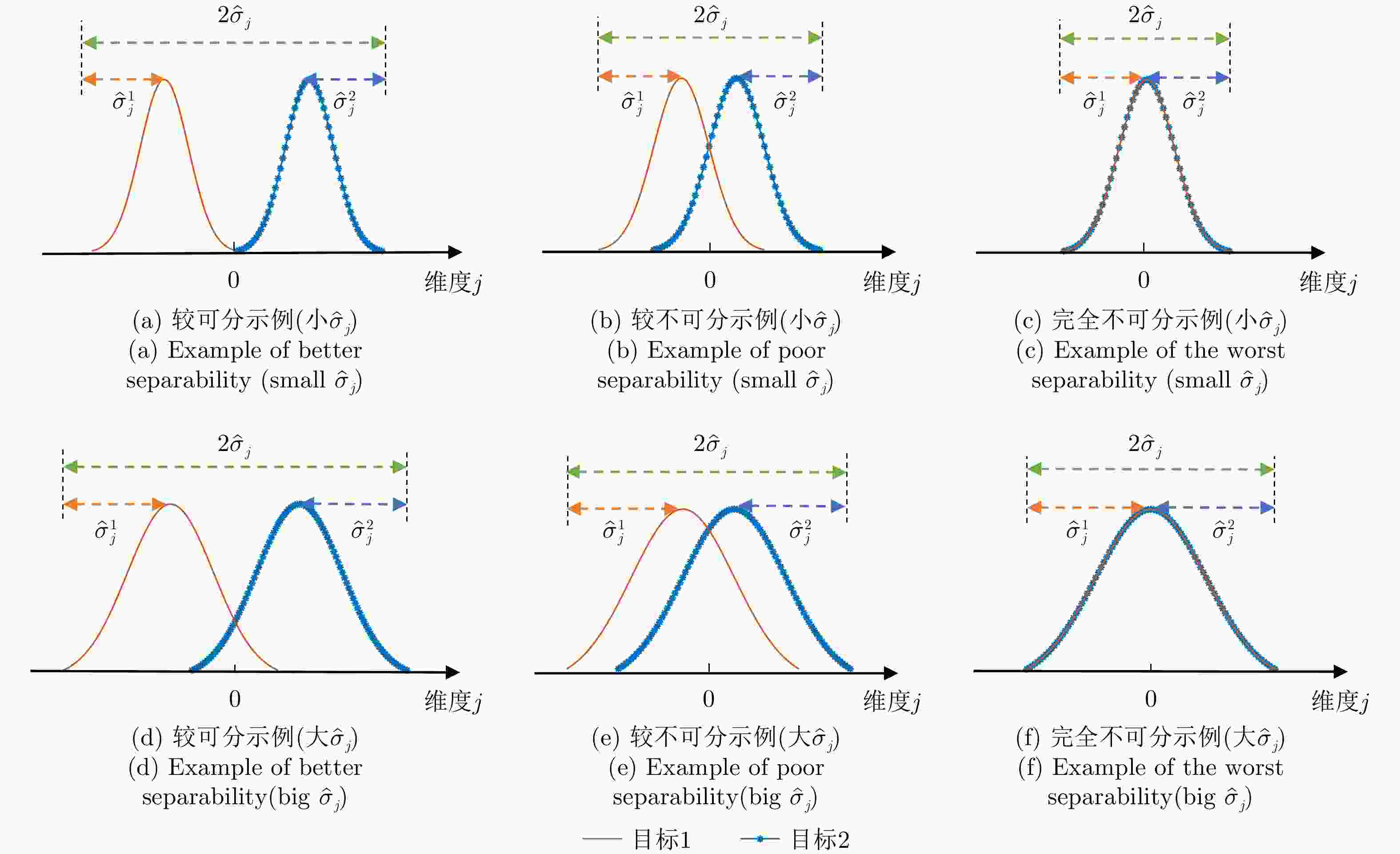
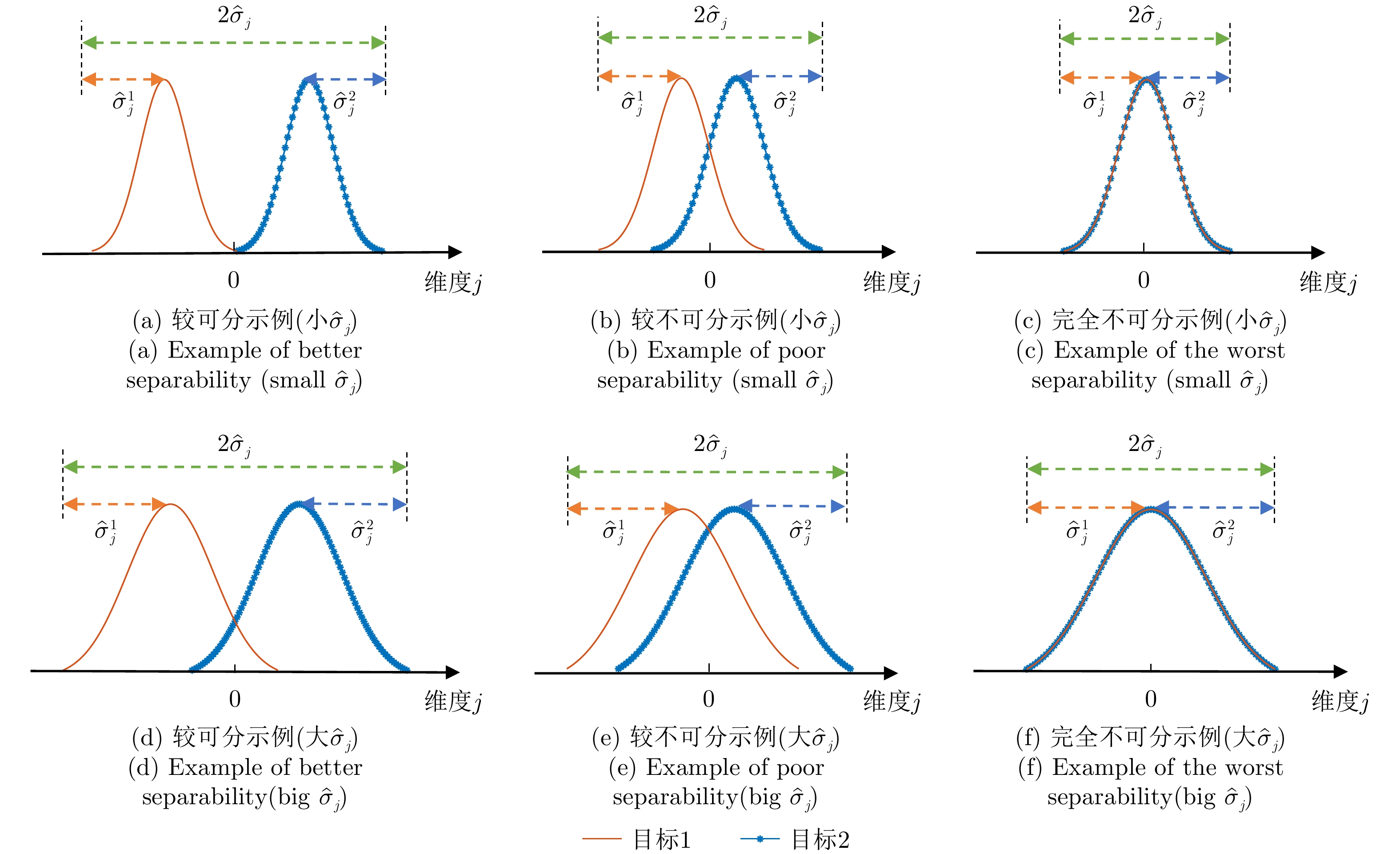
图 3 不同奇异值下的数据可分性示意图
Figure 3. Schematic of data separability under different singular values

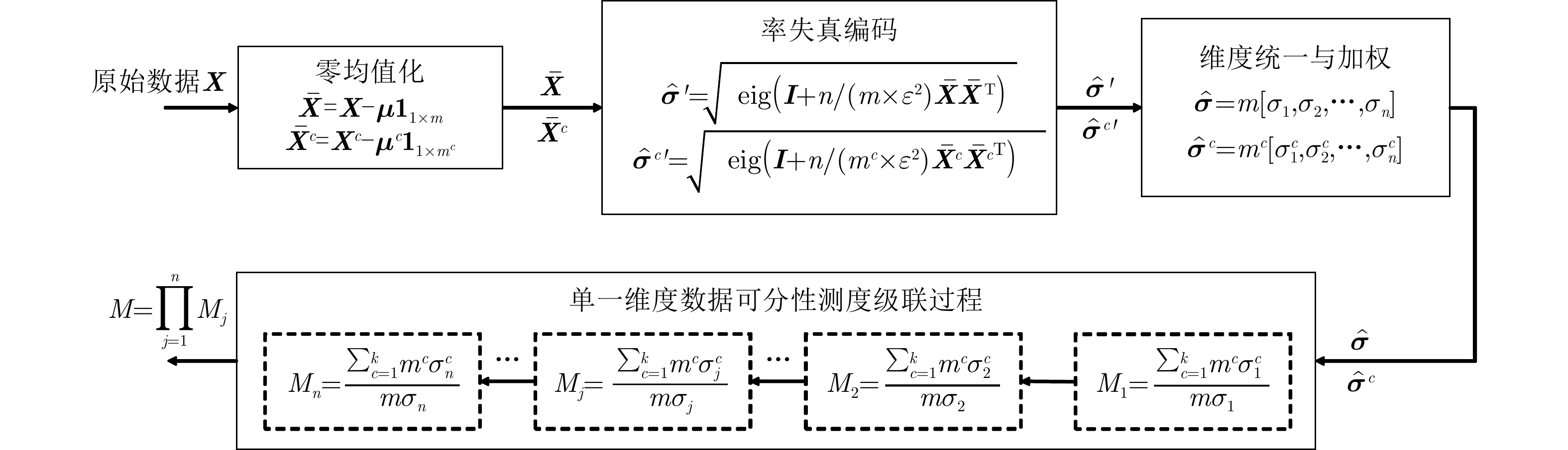
图 5 非高斯分布数据可分性度量构建示意图
Figure 5. Construction schematic of data separability measure under non-Gaussian condition
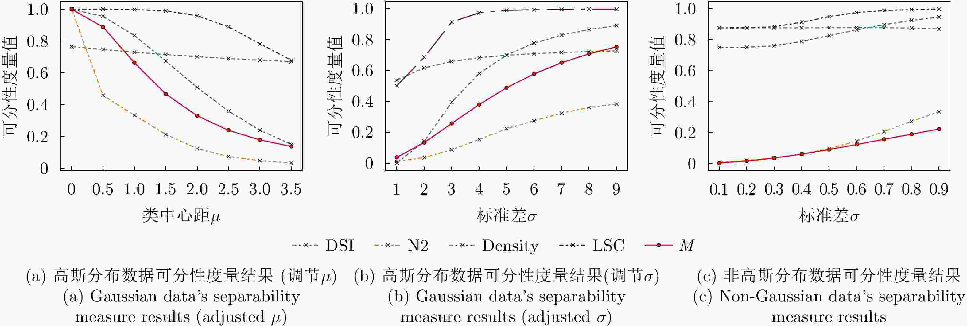
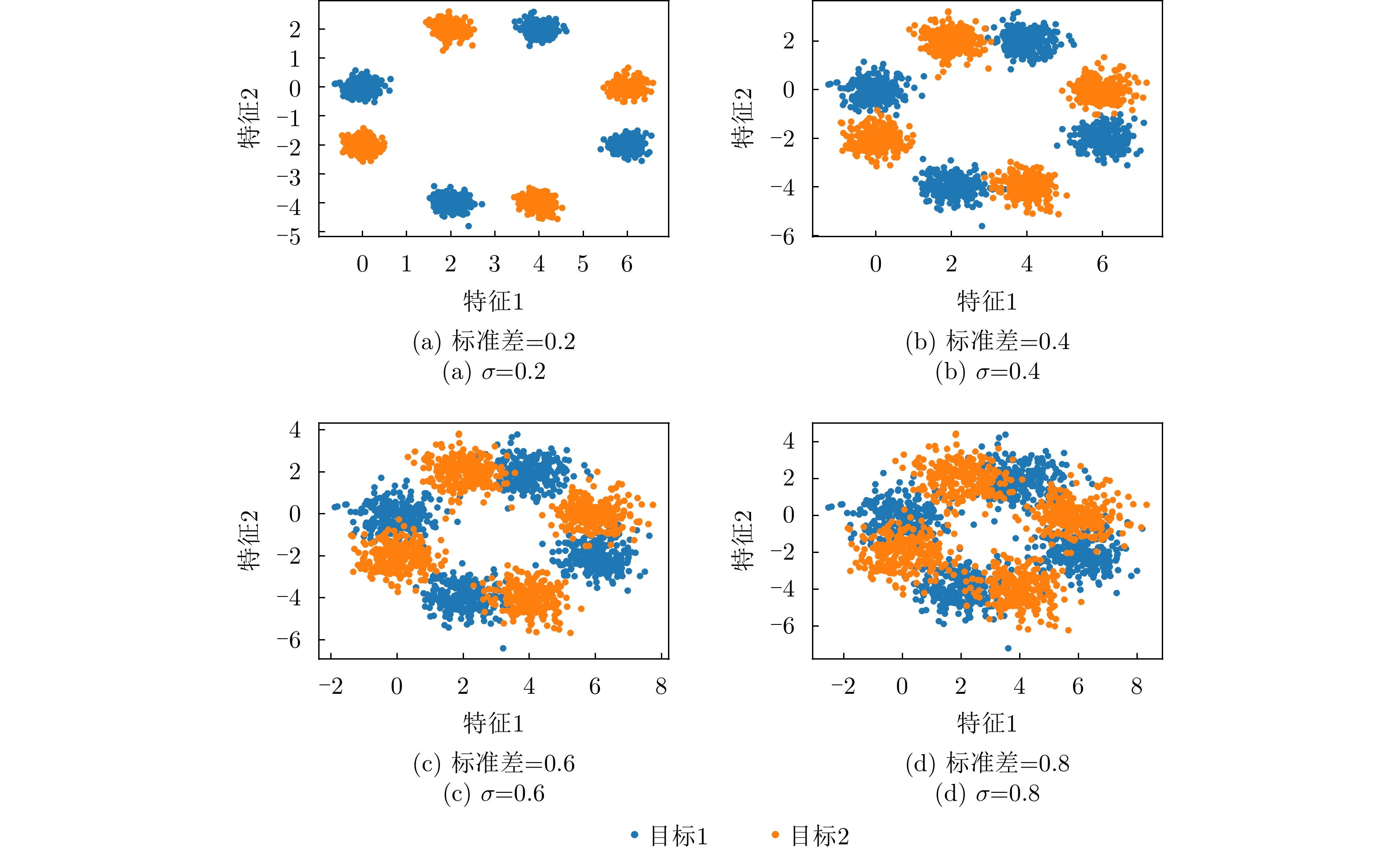
图 9 不同类间重叠度的数据可分性度量结果
Figure 9. Separability measures for datasets with different class overlap and dimensions

图 10 整体分布散度与类内分布散度变化趋势
Figure 10. The trend of overall and intra-class distribution divergence
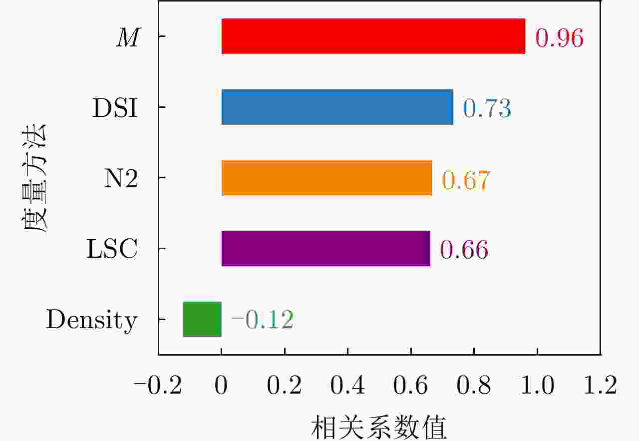
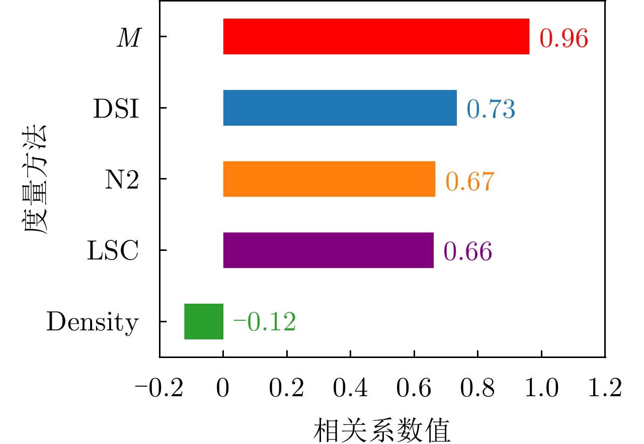
图 13 可分性度量与平均错误率相关性矩阵
Figure 13. Correlation matrix between separability measures and average recognition error

图 14 可分性度量与平均错误率曲线
Figure 14. Curves between separability measure and average recognition error
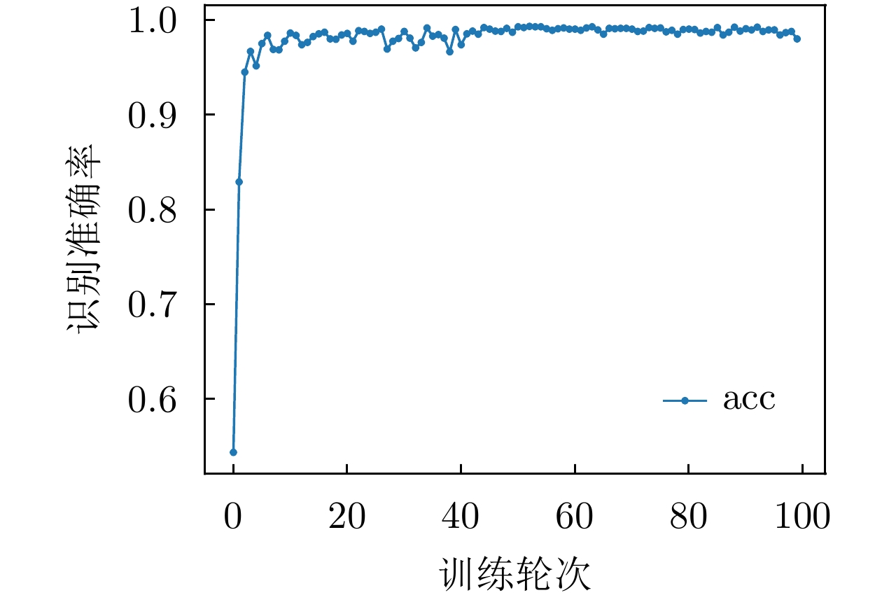
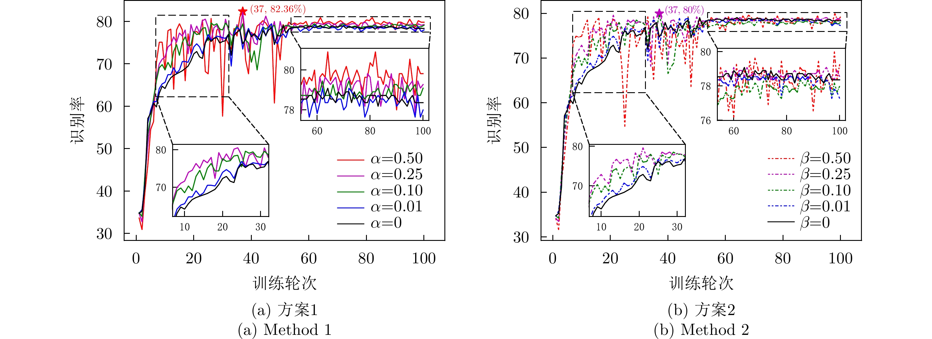
图 16 网络在MSTAR数据上的识别准确性能
Figure 16. Recognition accuracy performance of the network on MSTAR datasets
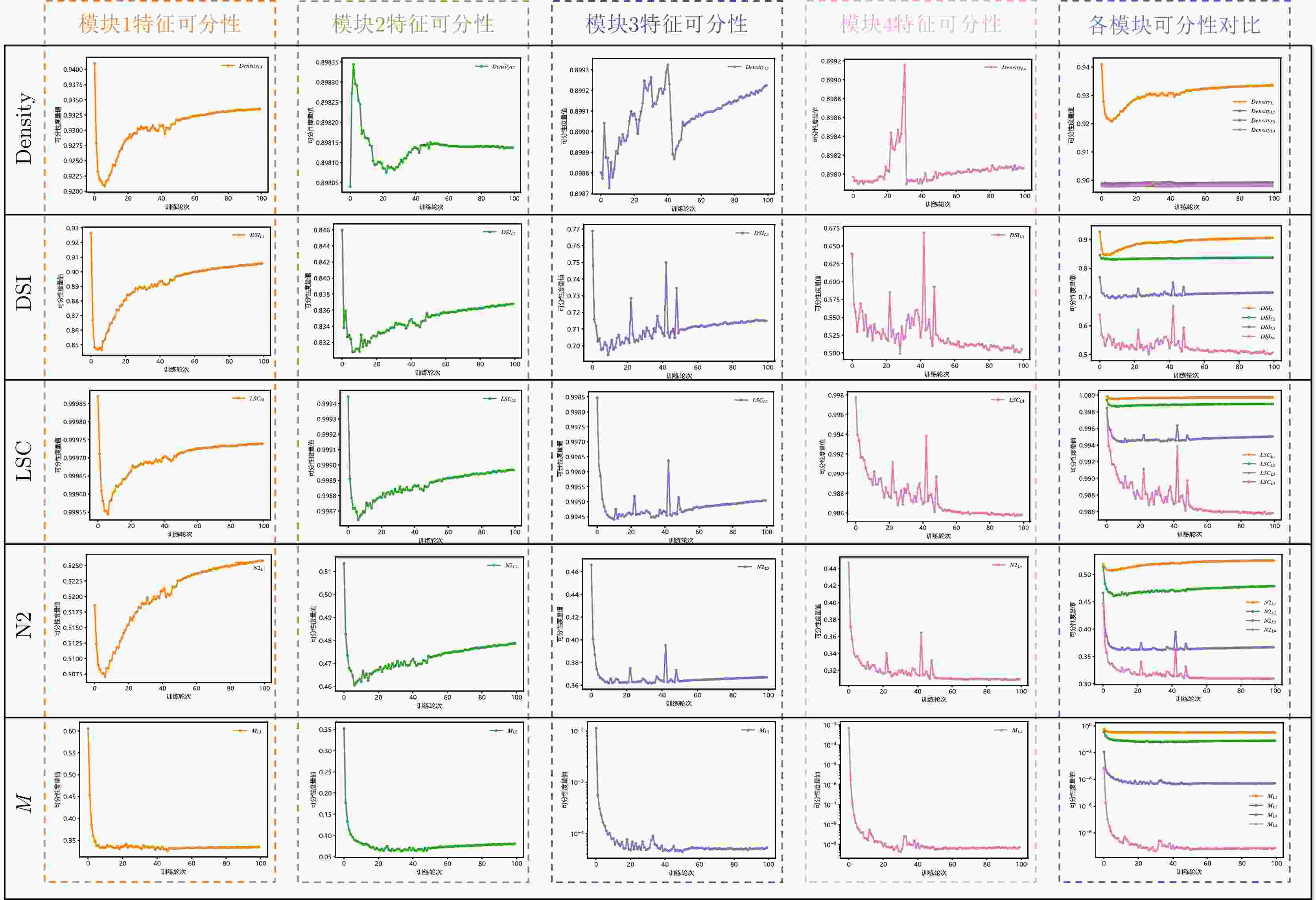
图 17 MSTAR数据集特征可分性度量结果
Figure 17. Feature separability measure results for MSTAR dataset

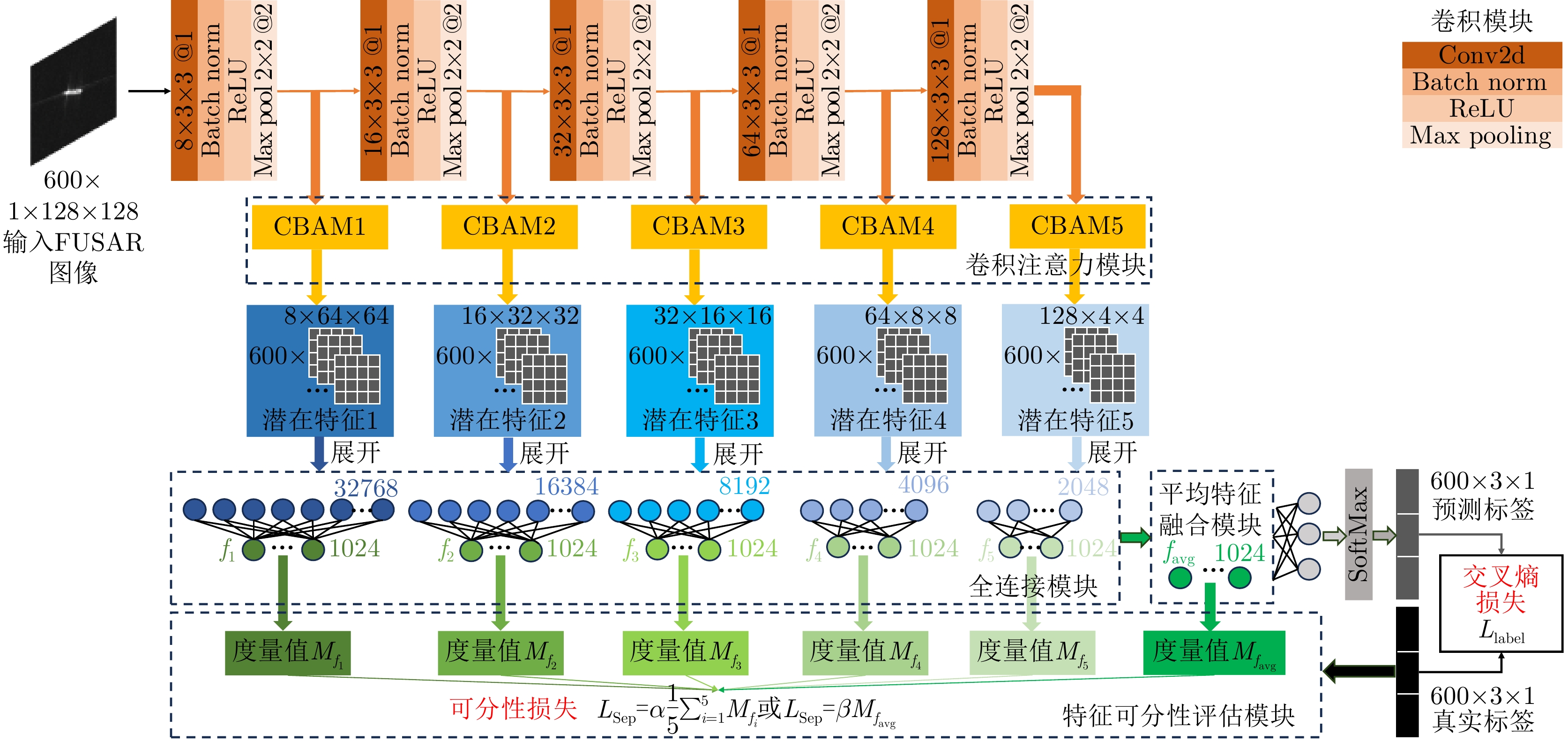
图 18 特征可分性度量约束下的卷积神经网络
Figure 18. Convolutional neural networks with feature separability constraints
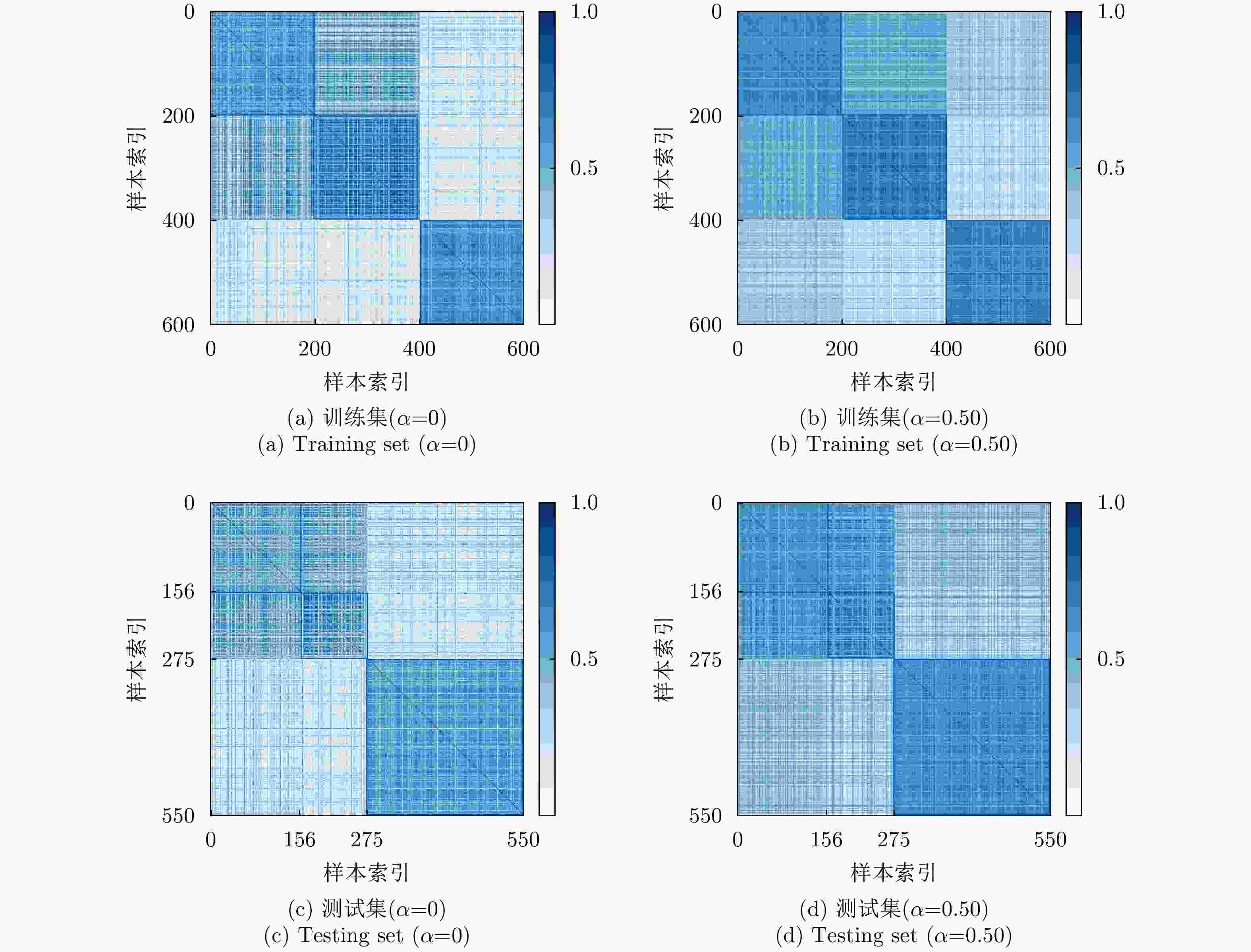
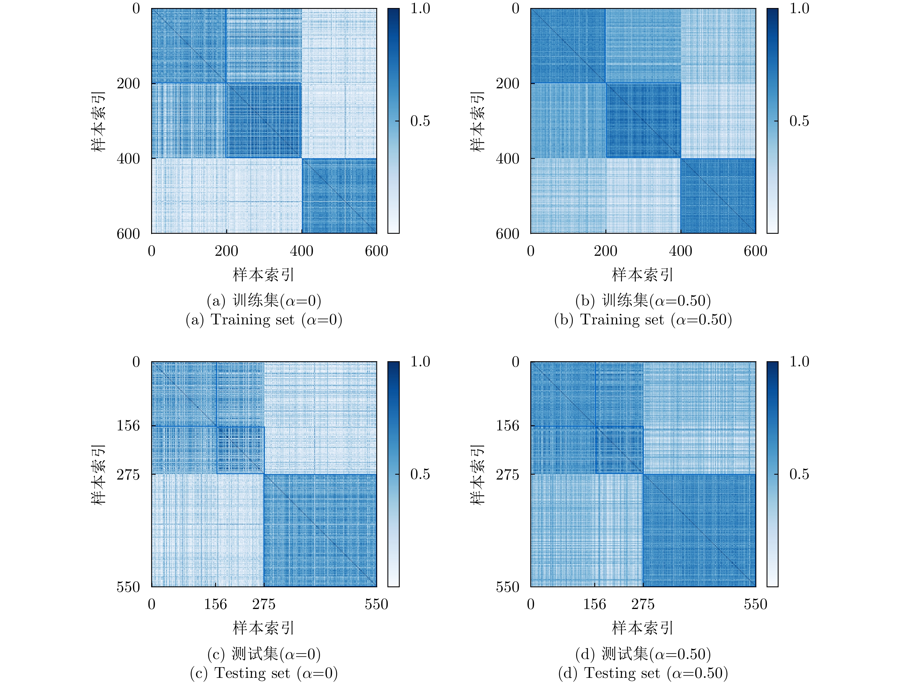
图 21 最终层输出特征样本间余弦相似度矩阵
Figure 21. The cosine similarity matrix between feature samples output from the final layer

图 22 最终层输出特征t-SNE图
Figure 22. The t-SNE visualization of the feature output from the final layer
1 平均意义下的数据可分性度量计算过程
1. Average data separability measure computing
1. 输入: 数据${\boldsymbol{X}} = \left\{ {{{\boldsymbol{X}}^c}} \right\}_{c = 1}^k$,聚类数${\boldsymbol{k}} = \left\{ {{k^c}} \right\}_{c = 1}^k$ 2. for $c = 1:k$执行 3. ${\text{GMM}}\left( {{{\boldsymbol{X}}^c},{k^c}} \right)$得到高斯子类,
$\left\{ {{{\boldsymbol{X}}^{1{c^1}}}} \right\}_{{c^1} = 1}^{{k^1}}$,$\left\{ {{{\boldsymbol{X}}^{2{c^2}}}} \right\}_{{c^2} = 1}^{{k^2}}$,···,$\left\{ {{{\boldsymbol{X}}^{k{c^k}}}} \right\}_{{c^k} = 1}^{{k^k}}$;4. end for 5. for $c = 1:k - 1$执行 6. for $t = c + 1:k$执行 7. for $i = 1:{k^c}$执行 8. for $j = 1:{k^t}$执行 9. 计算${M_{{\rm{citj}}} } = M\left( { { {\boldsymbol{X} }^{ci} },{ {\boldsymbol{X} }^{tj} } } \right)$ (根据式(15)); 10. 计算${N_{{\rm{citj}}} } = \left| { { {\boldsymbol{X} }^{ci} } } \right| + \left| { { {\boldsymbol{X} }^{tj} } } \right|$ ($\left| {\boldsymbol{X}} \right|$表示集合X的样本量); 11. end for 12. end for 13. end for 14. end for 15. 计算$\bar M = { { {\text{sum} }\left( { {M_{{\rm{citj}}} }{N_{{\rm{citj}}} } } \right)} \mathord{\left/ {\vphantom { { {\text{sum} }\left( { {M_{citj} }{N_{citj} } } \right)} { {\text{sum} }\left( { {N_{citj} } } \right)} } } \right. } { {\text{sum} }\left( { {N_{{\rm{citj}}} } } \right)} }$ (根据式(16)); 16. 输出: $\bar M$  下载: 导出CSV
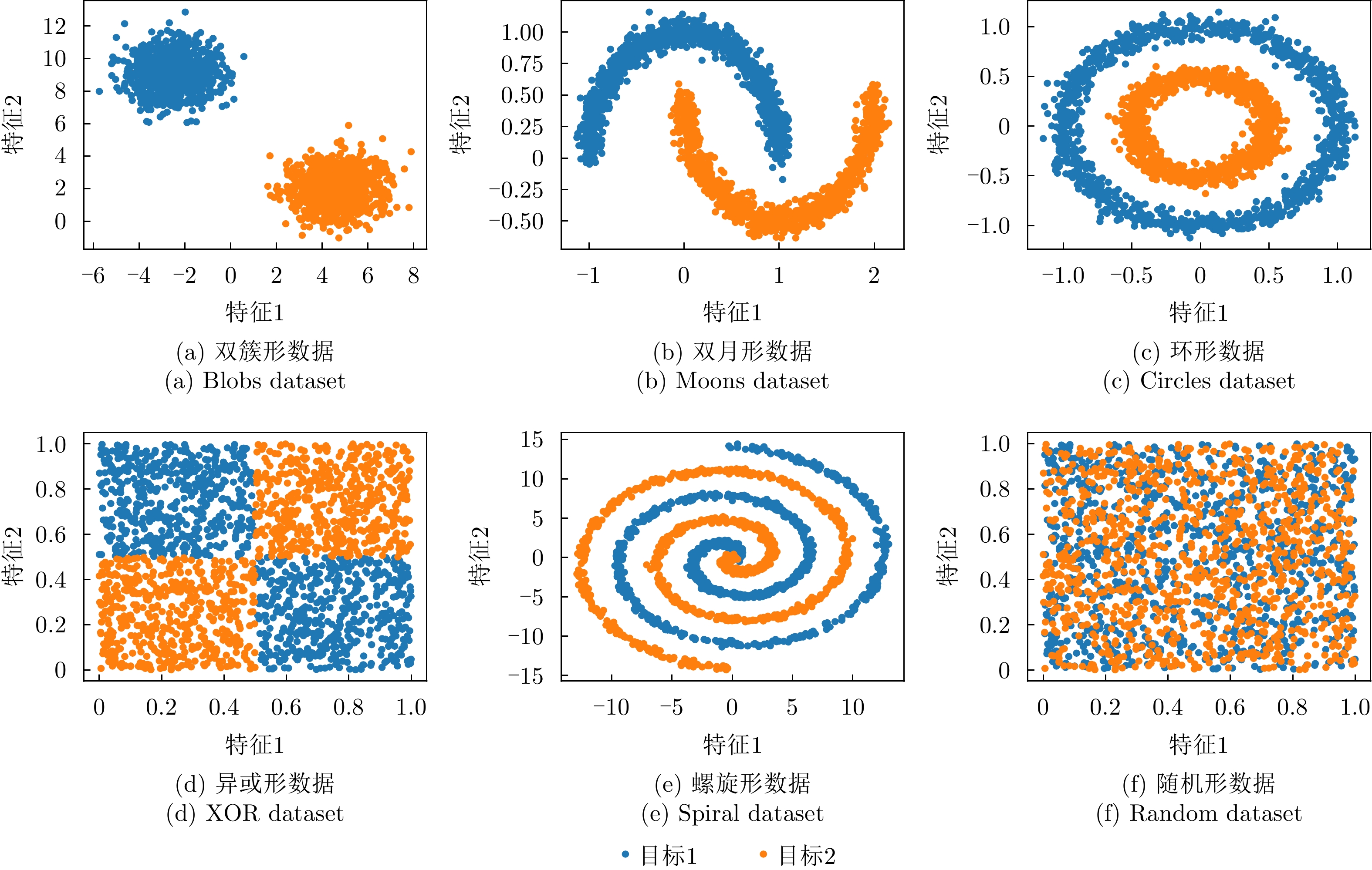
表 1 典型特征图可分性度量结果
Table 1. Separability measure results of typical feature
度量方法 双簇形 双月形 环形 异或形 螺旋形 混合形 DSI 0.0008 0.6459 0.5532 0.7775 0.9420 0.9941 N2 0.0110 0.0246 0.0461 0.0598 0.0569 0.4928 Density 0.5379 0.8322 0.8661 0.8857 0.8703 0.9282 LSC 0.5012 0.8362 0.9134 0.9148 0.9727 0.9994 $\bar M$(${k^1} = {k^2} = 1$) 0.0371 0.3305 0.9999 0.9995 0.9669 0.9990 $\bar M$(${k^1} = {k^2} = 3$) 0.0175 0.0592 0.1748 0.2216 0.5601 0.4823 $\bar M$(${k^1} = {k^2} = 5$) 0.0114 0.0262 0.0633 0.1449 0.3388 0.3461 $\bar M$(${k^1} = {k^2} = 8$) 0.0087 0.0164 0.0334 0.0911 0.2044 0.2482
下载: 导出CSV
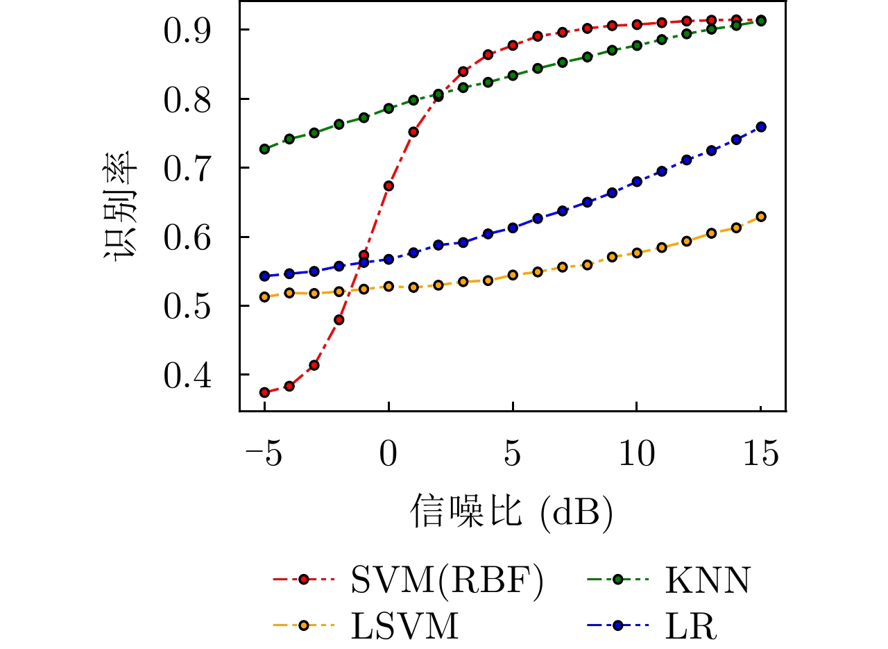
表 2 识别模型识别率结果
Table 2. Recognition accuracy results of recognition models
数据集 样本数(正例/负例) 特征数 SVM(RBF) KNN LSVM LR 平均识别率($\overline {{\text{Acc}}} $) Banknote 1372(762/610) 5 1.0000 1.0000 0.9879× 0.9879× 0.9939 Wisconsin 683(444/239) 9 0.9512× 0.9561 0.9561 0.9854√ 0.9622 WDBC 569(357/212) 30 0.9356 0.9591√ 0.9591√ 0.9181× 0.9430 Fire 244(138/106) 10 0.9189× 0.9190 0.9730√ 0.9190 0.9324 Ionosphere 351(225/126) 33 0.9623√ 0.8585× 0.8773 0.8773 0.8939 Spambase 4601(2788/1813) 57 0.6799 0.7820 0.8639√ 0.6618× 0.7469 Sonar 208(111/97) 60 0.8254 0.8413√ 0.8095 0.6984× 0.7936 Risk 776(486/290) 17 0.7425 0.8412 0.9184√ 0.6867× 0.7972 Mammographic 830(427/403) 5 0.7590 0.8032√ 0.7349× 0.7389 0.7590 Magic 19020(12332/6688) 10 0.8274√ 0.8098 0.6972 0.6008× 0.7338 Hill valley 606(305/301) 100 0.4780× 0.5385 0.9670√ 0.4780× 0.6154 Blood 748(570/178) 4 0.7378√ 0.7022 0.7333 0.6000× 0.6933 ILPD 583(416/167) 10 0.7314 0.6971 0.7428√ 0.6343× 0.7014 Haberman 306(225/81) 6 0.7174 0.7826√ 0.7065× 0.7391 0.7364 注:“√”表示其在对应行数据上识别率最高;“×”表示最低
下载: 导出CSV
表 3 实测数据集可分性度量结果
Table 3. Separability measure results of real data
数据集 样本数(正例/负例) N2 LSC Density DSI M 平均错误率($1 - \overline {{\text{Acc}}} $) Banknote 1372(762/610) 0.0883 0.9022 0.8027 0.7649 0.1355 0.0061 Wisconsin 683(444/239) 0.2491 0.6636 0.6203 0.3157 0.1567 0.0378 WDBC 569(357/212) 0.1380 0.9140 0.5630 0.5833 0.2497 0.0570 Fire 244(138/106) 0.2766 0.9103 0.7150 0.7058 0.2887 0.0676 Ionosphere 351(225/126) 0.3884 0.9118 0.8553 0.7177 0.3807 0.1061 Spambase 4601(2788/1813) 0.2553 0.9967 0.4780 0.8296 0.4402 0.2531 Sonar 208(111/97) 0.4079 0.9754 0.9333 0.9457 0.4497 0.2064 Risk 776(486/290) 0.2082 0.9471 0.7140 0.7894 0.5023 0.2028 Mammographic 830(427/403) 0.2681 0.9947 0.8045 0.8807 0.5813 0.2410 Magic 19020(12332/6688) – – – – 0.6742 0.2662 Hill valley 606(305/301) 0.4857 0.9981 0.6260 0.9727 0.7408 0.3846 Blood 748(570/178) 0.4379 0.9945 0.6235 0.9286 0.8678 0.3067 ILPD 583(416/167) 0.2988 0.9910 0.6732 0.8016 0.8800 0.2986 Haberman 306(225/81) 0.4428 0.9886 0.8279 0.9482 0.9102 0.2636
下载: 导出CSV
表 4 SAR图像数据集
Table 4. SAR image datasets
数据集 类别 训练集 测试集 数据集 类别 训练集 测试集 MSTAR BMP2 233 195 FUSAR 其余类别 200 275 BTR70 233 196 T72 232 196 BTR60 256 195 2S1 299 274 渔船 200 119 BRDM2 298 274 D7 299 274 T62 299 273 货船 200 156 ZIL131 299 274 ZSU234 299 274
下载: 导出CSV
表 5 不同可分性系数下最优识别率表现(%)
Table 5. Optimal accuracy performance with different separability factors (%)
系数 训练集识别率 测试集识别率 $\alpha = \beta = 0$(基准网络) 94.00 79.09 $\beta = 0.01$ 94.00 78.90 $\beta = 0.10$ 98.67 79.64 $\beta = 0.25$ 99.67 80.00 $\beta = 0.50$ 100.00 80.00 $\alpha = 0.01$ 93.83 79.45 $\alpha = 0.10$ 91.50 79.63 $\alpha = 0.25$ 98.17 82.18 $\alpha = 0.50$ 99.83 82.36
下载: 导出CSV
-
[1] 付强, 何峻. 自动目标识别评估方法及应用[M]. 北京, 科学出版社, 2013: 16–19.FU Qiang and HE Jun. Automatic Target Recognition Evaluation Method and its Application[M]. Beijing, Science Press, 2013: 16–19. [2] 郁文贤. 自动目标识别的工程视角述评[J]. 雷达学报, 2022, 11(5): 737–752. doi: 10.12000/JR22178YU Wenxian. Automatic target recognition from an engineering perspective[J]. Journal of Radars, 2022, 11(5): 737–752. doi: 10.12000/JR22178 [3] HOSSIN M and SULAIMAN M N. A review on evaluation metrics for data classification evaluations[J]. International Journal of Data Mining & Knowledge Management Process (IJDKP), 2015, 5(2): 1–11. doi: 10.5281/zenodo.3557376 [4] ZHANG Chiyuan, BENGIO S, HARDT M, et al. Understanding deep learning (still) requires rethinking generalization[J]. Communications of the ACM, 2021, 64(3): 107–115. doi: 10.1145/3446776 [5] OPREA M. A general framework and guidelines for benchmarking computational intelligence algorithms applied to forecasting problems derived from an application domain-oriented survey[J]. Applied Soft Computing, 2020, 89: 106103. doi: 10.1016/J.ASOC.2020.106103 [6] YU Shuang, LI Xiongfei, FENG Yuncong, et al. An instance-oriented performance measure for classification[J]. Information Sciences, 2021, 580: 598–619. doi: 10.1016/J.INS.2021.08.094 [7] FERNÁNDEZ A, GARCÍA S, GALAR M, et al. Learning from Imbalanced Data Sets[M]. Cham: Springer, 2018: 253–277. [8] BELLO M, NÁPOLES G, VANHOOF K, et al. Data quality measures based on granular computing for multi-label classification[J]. Information Sciences, 2021, 560: 51–57. doi: 10.1016/J.INS.2021.01.027 [9] CANO J R. Analysis of data complexity measures for classification[J]. Expert Systems with Applications, 2013, 40(12): 4820–4831. doi: 10.1016/J.ESWA.2013.02.025 [10] METZNER C, SCHILLING A, TRAXDORF M, et al. Classification at the accuracy limit: Facing the problem of data ambiguity[J]. Scientific Reports, 2022, 12(1): 22121. doi: 10.1038/S41598-022-26498-Z [11] 徐宗本. 人工智能的10个重大数理基础问题[J]. 中国科学: 信息科学, 2021, 51(12): 1967–1978. doi: 10.1360/SSI-2021-0254XU Zongben. Ten fundamental problems for artificial intelligence: Mathematical and physical aspects[J]. SCIENTIA SINICA Informationis, 2021, 51(12): 1967–1978. doi: 10.1360/SSI-2021-0254 [12] MISHRA A K. Separability indices and their use in radar signal based target recognition[J]. IEICE Electronics Express, 2009, 6(14): 1000–1005. doi: 10.1587/ELEX.6.1000 [13] GUAN Shuyue and LOEW M. A novel intrinsic measure of data separability[J]. Applied Intelligence, 2022, 52(15): 17734–17750. doi: 10.1007/S10489-022-03395-6 [14] BRUN A L, BRITTO A S JR, OLIVEIRA L S, et al. A framework for dynamic classifier selection oriented by the classification problem difficulty[J]. Pattern Recognition, 2018, 76: 175–190. doi: 10.1016/J.PATCOG.2017.10.038 [15] CHARTE D, CHARTE F, and HERRERA F. Reducing data complexity using autoencoders with class-informed loss functions[J]. IEEE Transactions on Pattern Analysis and Machine Intelligence, 2022, 44(12): 9549–9560. doi: 10.1109/TPAMI.2021.3127698 [16] LORENA A C, GARCIA L P F, LEHMANN J, et al. How complex is your classification problem?: A survey on measuring classification complexity[J]. ACM Computing Surveys, 2020, 52(5): 107. doi: 10.1145/3347711 [17] FERRARO M B and GIORDANI P. A review and proposal of (fuzzy) clustering for nonlinearly separable data[J]. International Journal of Approximate Reasoning, 2019, 115: 13–31. doi: 10.1016/J.IJAR.2019.09.004 [18] SHANNON C E. A mathematical theory of communication[J]. The Bell System Technical Journal, 1948, 27(3): 379–423. doi: 10.1002/J.1538-7305.1948.TB01338.X [19] COVER T M and THOMAS J A. Elements of Information Theory[M]. New York: Wiley, 1991: 301–332. [20] MADIMAN M, HARRISON M, and KONTOYIANNIS I. Minimum description length vs. maximum likelihood in lossy data compression[C]. 2004 International Symposium on Information Theory, Chicago, USA, 2004: 461. [21] MA Yi, DERKSEN H, HONG Wei, et al. Segmentation of multivariate mixed data via lossy data coding and compression[J]. IEEE Transactions on Pattern Analysis and Machine Intelligence, 2007, 29(9): 1546–1562. doi: 10.1109/TPAMI.2007.1085 [22] MACDONALD J, WÄLDCHEN S, HAUCH S, et al. A rate-distortion framework for explaining neural network decisions[J]. arXiv: 1905.11092, 2019. [23] HAN Xiaotian, JIANG Zhimeng, LIU Ninghao, et al. Geometric graph representation learning via maximizing rate reduction[C]. ACM Web Conference, Lyon, France, 2022: 1226–1237. [24] CHOWDHURY S B R and CHATURVEDI S. Learning fair representations via rate-distortion maximization[J]. Transactions of the Association for Computational Linguistics, 2022, 10: 1159–1174. doi: 10.1162/TACL_A_00512 [25] LICHMAN M E A. Uci machine learning reposit[EB/OL]. https://archive.ics.uci.edu/datasets, 2023. [26] HO T K and BASU M. Complexity measures of supervised classification problems[J]. IEEE Transactions on Pattern Analysis and Machine Intelligence, 2002, 24(3): 289–300. doi: 10.1109/34.990132 [27] LEYVA E, GONZÁLEZ A, and PÉREZ R. A set of complexity measures designed for applying meta-learning to instance selection[J]. IEEE Transactions on Knowledge and Data Engineering, 2015, 27(2): 354–367. doi: 10.1109/TKDE.2014.2327034 [28] GARCIA L P F, DE CARVALHO A C P L F, and LORENA A C. Effect of label noise in the complexity of classification problems[J]. Neurocomputing, 2015, 160: 108–119. doi: 10.1016/J.NEUCOM.2014.10.085 [29] AGGARWAL C C, HINNEBURG A, and KEIM D A. On the surprising behavior of distance metrics in high dimensional space[C]. 8th International Conference on Database Theory, London, UK, 2001: 420–434. [30] MILLER K, MAURO J, SETIADI J, et al. Graph-based active learning for semi-supervised classification of SAR data[C]. SPIE 12095, Algorithms for Synthetic Aperture Radar Imagery XXIX, Orlando, United States, 2022: 120950C. [31] 雷禹, 冷祥光, 孙忠镇, 等. 宽幅SAR海上大型运动舰船目标数据集构建及识别性能分析[J]. 雷达学报, 2022, 11(3): 347–362. doi: 10.12000/JR21173LEI Yu, LENG Xiangguang, SUN Zhongzhen, et al. Construction and recognition performance analysis of wide-swath SAR maritime large moving ships dataset[J]. Journal of Radars, 2022, 11(3): 347–362. doi: 10.12000/JR21173 [32] HOU Xiyue, AO Wei, SONG Qian, et al. FUSAR-Ship: Building a high-resolution SAR-AIS matchup dataset of Gaofen-3 for ship detection and recognition[J]. Science China Information Sciences, 2020, 63(4): 140303. doi: 10.1007/s11432-019-2772-5 [33] KEYDEL E R, LEE S W, and MOORE J T. MSTAR extended operating conditions: A tutorial[C]. SPIE 2757, Algorithms for Synthetic Aperture Radar Imagery III, Orlando, USA, 1996: 228–242. [34] CHEN Sizhe, WANG Haipeng, XU Feng, et al. Target classification using the deep convolutional networks for SAR images[J]. IEEE Transactions on Geoscience and Remote Sensing, 2016, 54(8): 4806–4817. doi: 10.1109/TGRS.2016.2551720 [35] ZHANG Tianwen, ZHANG Xiaoling, KE Xiao, et al. HOG-ShipCLSNet: A novel deep learning network with HOG feature fusion for SAR ship classification[J]. IEEE Transactions on Geoscience and Remote Sensing, 2022, 60: 5210322. doi: 10.1109/TGRS.2021.3082759 -


计量
- 文章访问数:
- HTML全文浏览量:
- PDF下载量:
- 被引次数: 0

