
 作者中心
作者中心 专家审稿
专家审稿 责编办公
责编办公 编辑办公
编辑办公
High-resolution Sparse Self-calibration Imaging for Vortex Radar with Phase Error
DOI: 10.12000/JR21094 cstr: 32380.14.JR21094
-
摘要:
基于轨道角动量(OAM)的涡旋雷达因其在高分辨率成像方面具有巨大潜力而受到广泛关注。有限OAM模式下的涡旋雷达高分辨率成像问题,通常采用稀疏恢复的方法来解决,这种方法需要精确地已知成像模型的先验知识。然而,系统中不可避免存在的相位误差,会导致成像模型失配,严重影响成像性能。为了解决这一问题,该文首次建立了存在相位误差时的涡旋雷达成像模型。同时,提出了一种涡旋雷达两步自校正成像方法,用于直接估计相位误差。首先在第1步中提出了一种稀疏驱动算法来促进目标稀疏性,同时提升成像重构性能。其次,在第2步中提出了一种直接补偿相位误差的自校正操作。该方法通过对目标重构和相位误差估计的交替迭代,能够很好地重建目标并有效地补偿相位误差。仿真结果表明,该方法在提高成像质量和改善相位误差估计性能方面具有潜在的优势。
Abstract:The Orbital Angular Momentum (OAM)-based vortex radar has drawn increasing attention because of its potential for high-resolution imaging. The vortex radar high resolution imaging with limited OAM modes is commonly solved by sparse recovery, in which the prior knowledge of the imaging model needs to be known precisely. However, the inevitable phase error in the system results in imaging model mismatch and deteriorates the imaging performance considerably. To address this problem, the vortex radar imaging model with phase error is established for the first time in this work. Meanwhile, a two-step self-calibration imaging method for vortex radar is proposed to directly estimate the phase error. In the first step, a sparsity-driven algorithm is developed to promote sparsity and improve imaging performance. In the second step, a self-calibration operation is performed to directly compensate for the phase error. By alternately reconstructing the targets and estimating the phase error, the proposed method can reconstruct the target with high imaging quality and effectively compensate for the phase error. Simulation results demonstrate the advantages of the proposed method in enhancing the imaging quality and improving the phase error estimation performance.
-
Key words:
- Vortex radar imaging /
- Orbital Angular Momentum (OAM) /
- Phase error /
- Self-calibration /
- Sparse recovery
-

Figure 3. In mode number [–10, 10], the obtained vortex EM images with phase error using different algorithms for SNR=20 dB
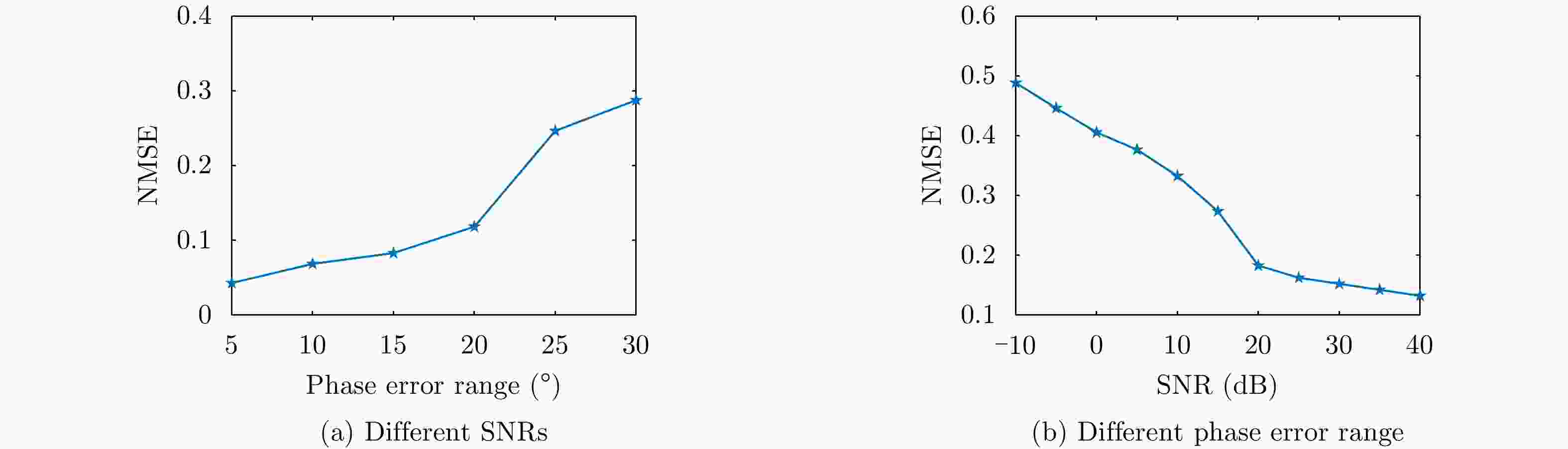
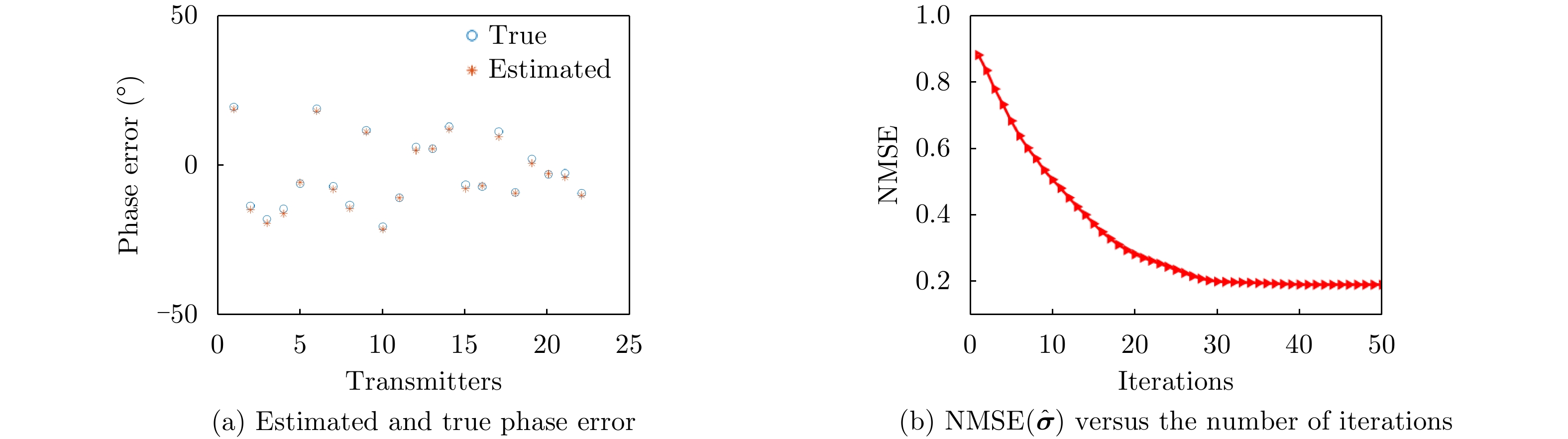
Figure 5.
${\rm{NMSE}}({\hat{\boldsymbol \beta }})$ of phase error under different SNRs and different phase error range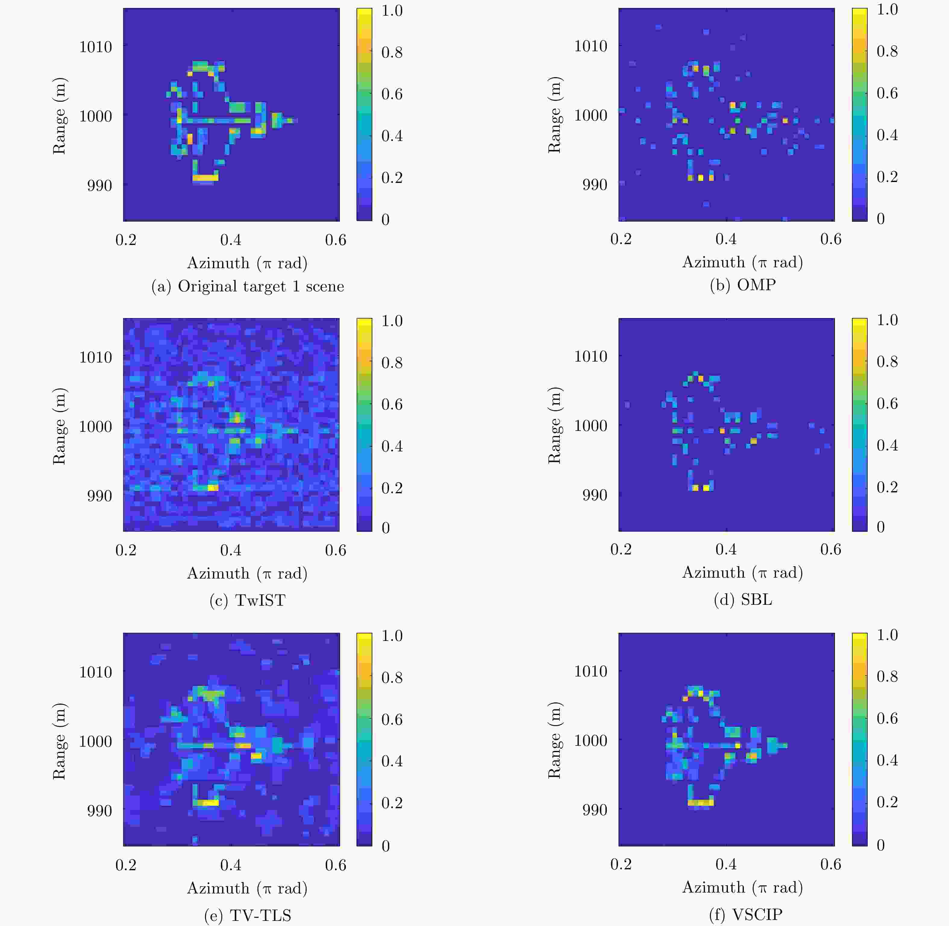
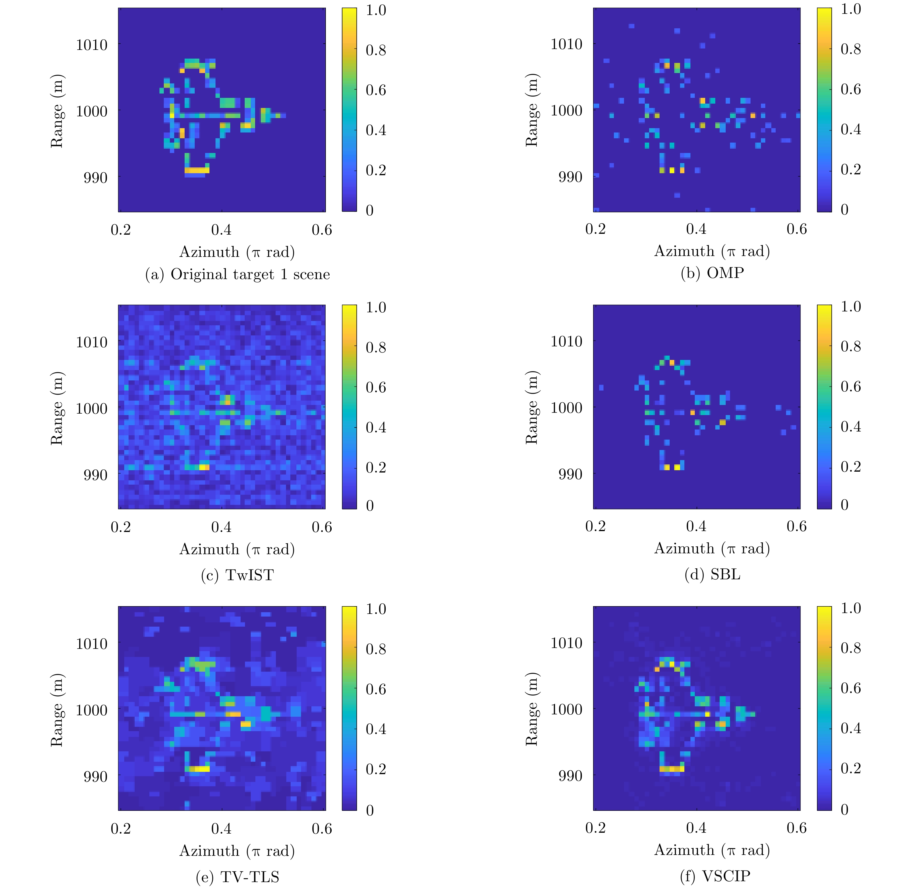
Figure 6. In mode number [–10, 10], the obtained vortex EM images of target 1 scene with phase error using different algorithms for SNR=5 dB
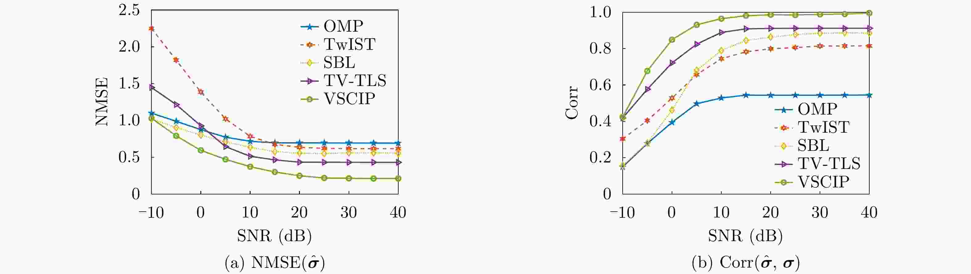
Figure 7. Under different SNRs, and obtained of original target 1 scene in mode number [–10, 10]

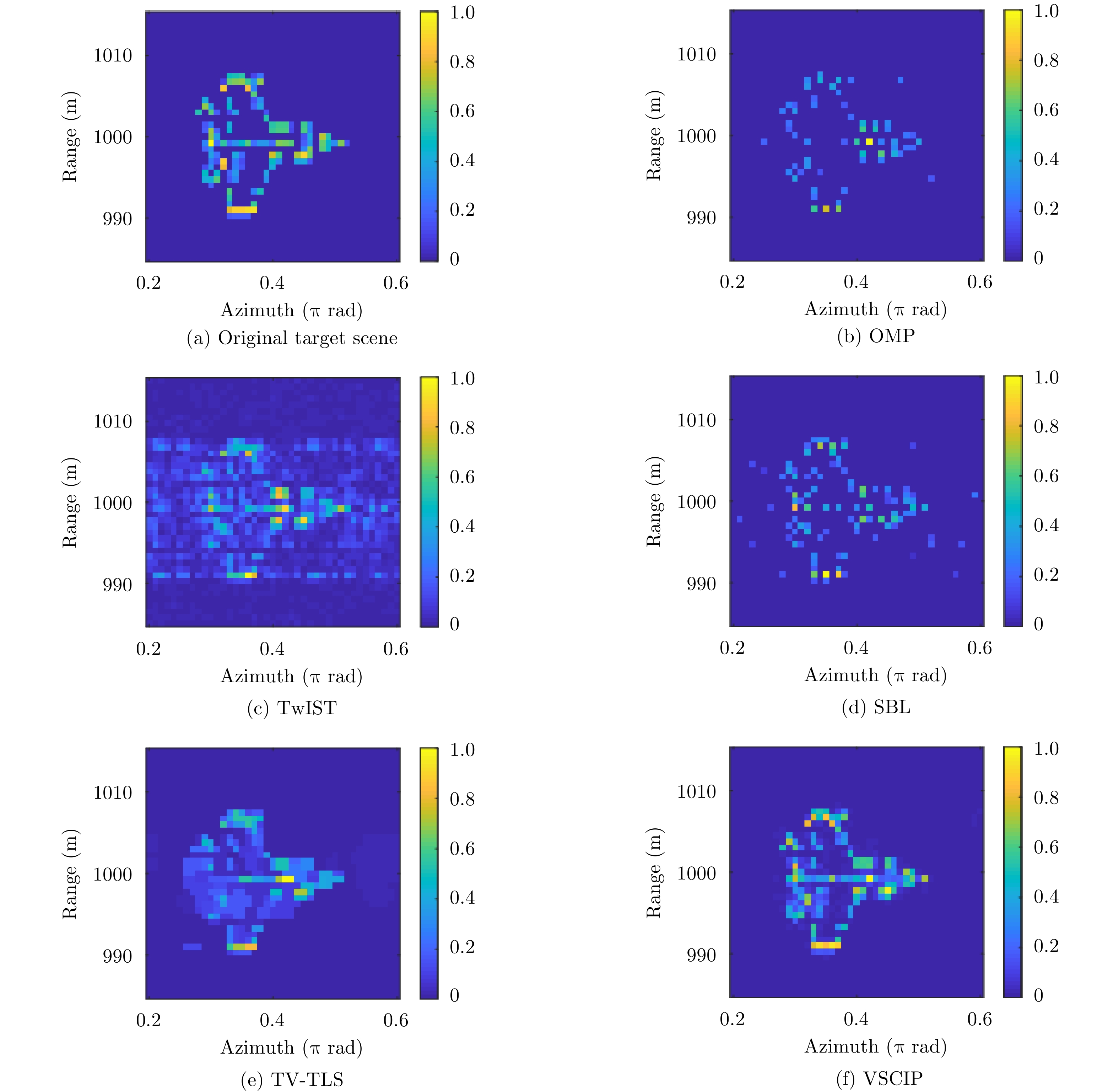
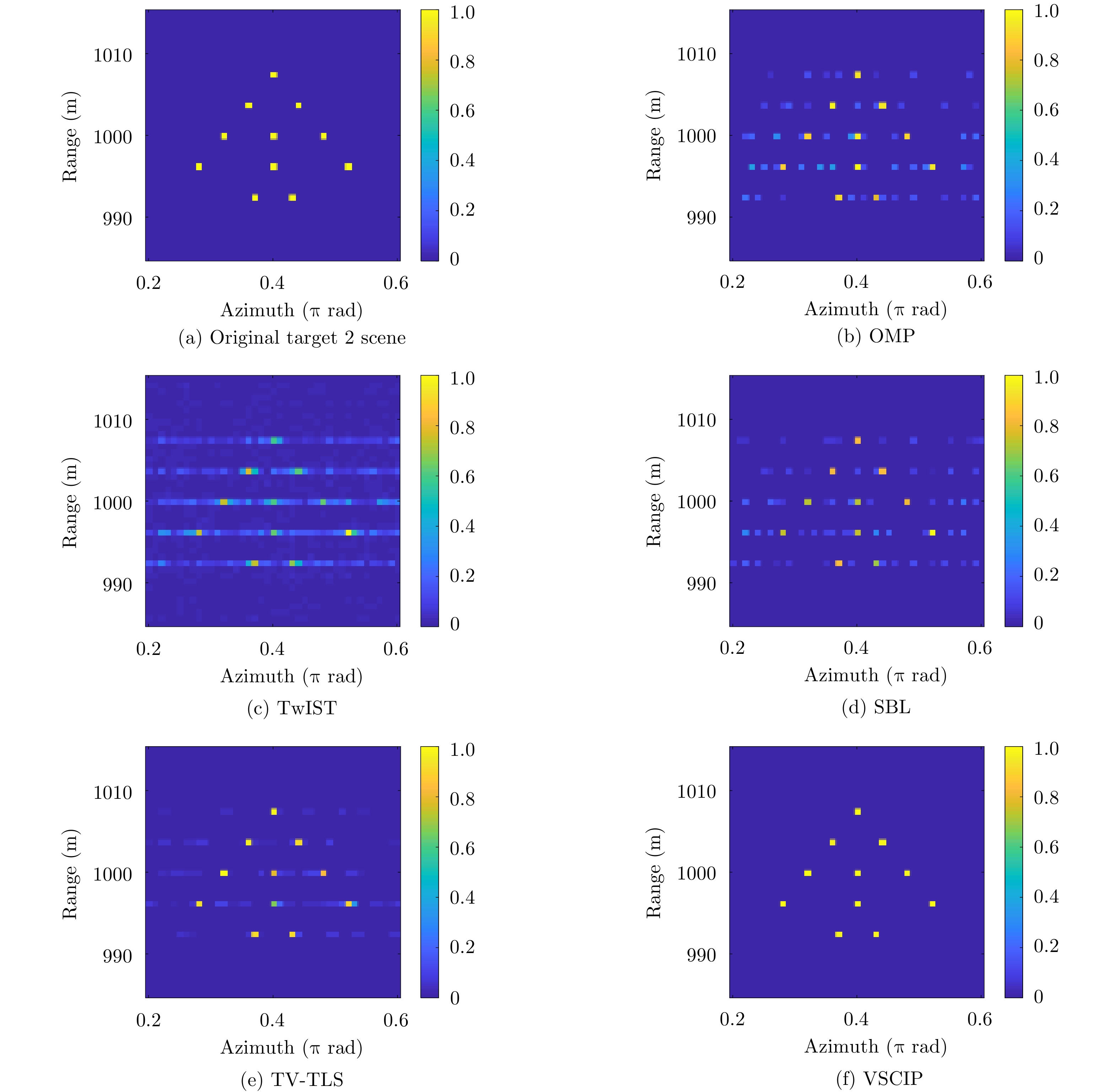
Figure 8. In mode number [–10, 10], the obtained vortex EM images of target 2 scene with phase error using different algorithms for SNR=20 dB

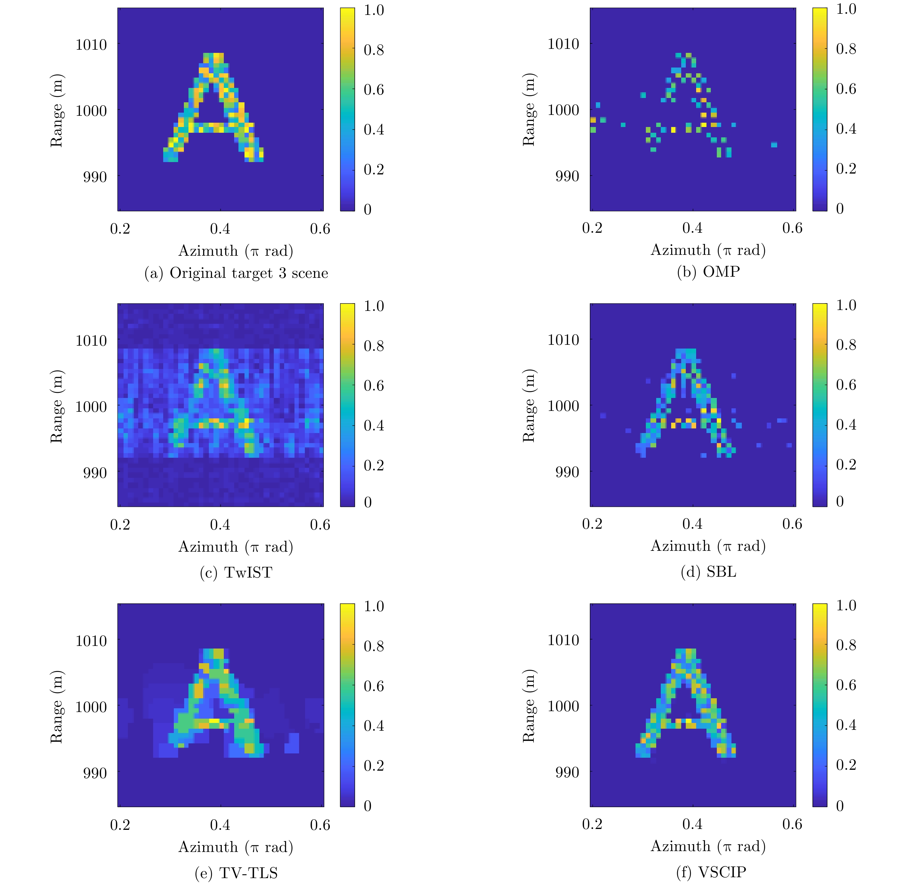
Figure 9. In mode number [–10, 10], the obtained vortex EM images of target 3 scene with phase error using different algorithms for SNR=20 dB
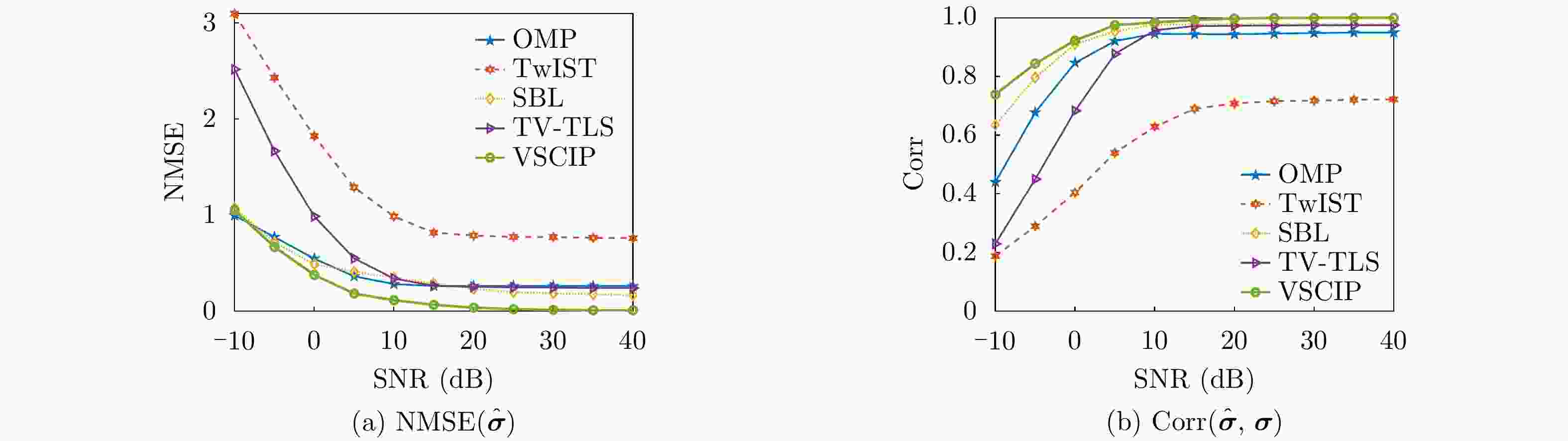
Figure 10. Under different SNRs,
${\rm{NMSE}}({{\boldsymbol{\hat{\sigma}} }})$ and${\rm{Corr}}({{\boldsymbol{\hat{\sigma }}}},\,{\boldsymbol{\sigma }})$ obtained of original target 2 scene in mode number [–10, 10]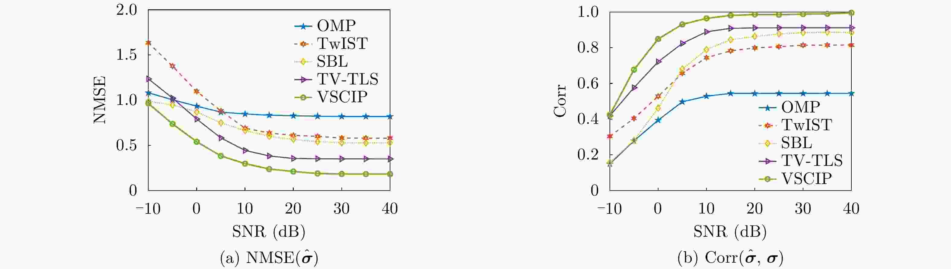
Figure 11. Under different SNRs,
${\rm{NMSE}}({{\boldsymbol{\hat{\sigma }}}})$ and${\rm{Corr}}({\boldsymbol{{\hat{\sigma }}}},\,{\boldsymbol{\sigma }})$ obtained of original target 3 scene in mode number [–10, 10]Algorithm 1 Algorithm flow of VSCIP Input: $ {{\boldsymbol{y}},{\boldsymbol{S}}},\epsilon,{a}_{0},{b}_{0}$ Initialization: ${\boldsymbol{\zeta } } = {\boldsymbol{1} },{\boldsymbol{\mu } } = { {\boldsymbol{S} }^{\rm{H}}}{\boldsymbol{y} }$ While $j < {j_{\max }}$ do For $t = 1$ to ${t_{\max }}$ do Update ${{\boldsymbol{\mu }}^j}$ and ${{\boldsymbol{\varSigma }}^j}$ by Eqs. (30) and (29); Update ${{\boldsymbol{\lambda }}^j}$ by Eq. (39); Update $\left\langle {\ln {\pi _m} } \right\rangle$ and $\left\langle {\ln \left( {1 - {\pi _m} } \right)} \right\rangle$ by Eqs. (42) and (43); Update ${{\boldsymbol{\zeta }}^j}$ by Eq. (50); Update ${\eta ^j}$ by Eq. (46); If $\left\| { { {\hat {\boldsymbol{\mu } } }^j}(t + 1) - { {\hat {\boldsymbol{\mu } } }^j}(t)} \right\|_2^2/\left\| {\hat {\boldsymbol{\mu } }{ {(t)}^j} } \right\|_2^2 < \epsilon$, break; ${{\boldsymbol{x}}^j} = {{\boldsymbol{\mu }}^j}(t + 1),{{\boldsymbol{w}}^j} = {{\boldsymbol{w}}^j}(t + 1)$; ${{\boldsymbol{\sigma }}^j}={{\boldsymbol{x}}^j} \odot {{\boldsymbol{w}}^j}$; End For Update ${{\boldsymbol{\beta }}^j}$ by Eq. (53); Recompute ${\boldsymbol{S}}({{\boldsymbol{\beta }}^j})$; End While Output: ${{\boldsymbol{\sigma }}^j}$, ${{\boldsymbol{\beta }}^j}$  下载: 导出CSV
Table 1. Key radar parameters for simulations
Parameters Value Frequency of the first subpulse $ f_0 $ 9.9 GHz Bandwith $B_r $ 200 MHz Number of subpulse $D $ 41 Topological charge $ \alpha $ [–10, 10] Array radius $a $ 0.25 m Array elements number N 22 Target range (985, 1015) m Target azimuth (0.2, 0.6)π rad
下载: 导出CSV
-
[1] MOHAMMADI S M, DALDORFF L K S, BERGMAN J E S, et al. Orbital angular momentum in radio—A system study[J]. IEEE Transactions on Antennas and Propagation, 2010, 58(2): 565–572. doi: 10.1109/tap.2009.2037701 [2] ALLEN L, BEIJERSBERGEN M W, SPREEUW R J C, et al. Orbital angular momentum of light and the transformation of Laguerre-Gaussian laser modes[J]. Physical Review A, 1992, 45(11): 8185–8189. doi: 10.1103/physreva.45.8185 [3] ZHANG Hengkang, ZHANG Bin, and LIU Qiang. OAM-basis transmission matrix in optics: A novel approach to manipulate light propagation through scattering media[J]. Optics Express, 2020, 28(10): 15006–15015. doi: 10.1364/OE.393396 [4] ZHANG Zhuofan, ZHENG Shilie, CHEN Yiling, et al. The capacity gain of orbital angular momentum based multiple-input-multiple-output system[J]. Scientific Reports, 2016, 6: 25418. doi: 10.1038/srep25418 [5] ZHAO Yufei and ZHANG Chao. Distributed antennas scheme for orbital angular momentum long-distance transmission[J]. IEEE Antennas and Wireless Propagation Letters, 2020, 19(2): 332–336. doi: 10.1109/lawp.2019.2962199 [6] GUO Guirong, HU Weidong, and DU Xiaoyong. Electromagnetic vortex based radar target imaging[J]. Journal of National University of Defense Technology, 2013, 35(6): 71–76. doi: 10.3969/j.issn.1001-2486.2013.06.013 [7] LIU Kang, CHENG Yongqiang, YANG Zhaocheng, et al. Orbital-angular-momentum-based electromagnetic vortex imaging[J]. IEEE Antennas and Wireless Propagation Letters, 2015, 14: 711–714. doi: 10.1109/lawp.2014.2376970 [8] LIN Mingtuan, GAO Yue, LIU Peiguo, et al. Super-resolution orbital angular momentum based radar targets detection[J]. Electronics Letters, 2016, 52(13): 1168–1170. doi: 10.1049/el.2016.0237 [9] LIU Kang, CHENG Yongqiang, LI Xiang, et al. Generation of orbital angular momentum beams for electromagnetic vortex imaging[J]. IEEE Antennas and Wireless Propagation Letters, 2016, 15: 1873–1876. doi: 10.1109/LAWP.2016.2542187 [10] LIN Mingtuan, GAO Yue, LIU Peiguo, et al. Theoretical analyses and design of circular array to generate orbital angular momentum[J]. IEEE Transactions on Antennas and Propagation, 2017, 65(7): 3510–3519. doi: 10.1109/tap.2017.2700160 [11] ZHANG Chao, JIANG Xuefeng, and CHEN Dong. Signal-to-noise ratio improvement by vortex wave detection with a rotational antenna[J]. IEEE Transactions on Antennas and Propagation, 2021, 69(2): 1020–1029. doi: 10.1109/TAP.2020.3016173 [12] LAVERY M P J, SPEIRITS F C, BARNETT S M, et al. Detection of a spinning object using light’s orbital angular momentum[J]. Science, 2013, 341(6145): 537–540. doi: 10.1126/science.1239936 [13] WANG Yu, LIU Kang, LIU Hongyan, et al. Detection of rotational object in arbitrary position using vortex electromagnetic waves[J]. IEEE Sensors Journal, 2021, 21(4): 4989–4994. doi: 10.1109/jsen.2020.3032665 [14] QIN Yuliang, LIU Kang, CHENG Yongqiang, et al. Sidelobe suppression and beam collimation in the generation of vortex electromagnetic waves for radar imaging[J]. IEEE Antennas and Wireless Propagation Letters, 2017, 16: 1289–1292. doi: 10.1109/LAWP.2016.2633008 [15] LIU Kang, CHENG Yongqiang, WANG Hongqiang, et al. Radiation pattern synthesis for the generation of vortex electromagnetic wave[J]. IET Microwaves, Antennas & Propagation, 2017, 11(5): 685–694. doi: 10.1049/iet-map.2016.0681 [16] LIU Kang, LI Xiang, GAO Yue, et al. High-resolution electromagnetic vortex imaging based on sparse bayesian learning[J]. IEEE Sensors Journal, 2017, 17(21): 6918–6927. doi: 10.1109/JSEN.2017.2754554 [17] QU Haiyou, CHENG Di, CHEN Chang, et al. Sparsity-driven high-resolution fast electromagnetic vortex imaging based on two-dimensional NCALM[C]. 2020 IEEE 6th International Conference on Computer and Communications, Chengdu, China, 2020. doi: 10.1109/iccc51575.2020.9345020. [18] WANG Lin, TAO Lujing, LI Zhongyu, et al. A new air target orientation observations based on electromagnetic vortex radar[C]. The 6th Asia-Pacific Conference on Synthetic Aperture Radar, Xiamen, China, 2019. doi: 10.1109/apsar46974.2019.9048450. [19] HE Qian and BLUM R S. Cramer-rao bound for MIMO radar target localization with phase errors[J]. IEEE Signal Processing Letters, 2010, 17(1): 83–86. doi: 10.1109/LSP.2009.2032994 [20] YANG Yang and BLUM R S. Phase synchronization for coherent MIMO radar: Algorithms and their analysis[J]. IEEE Transactions on Signal Processing, 2011, 59(11): 5538–5557. doi: 10.1109/TSP.2011.2162509 [21] LI Jun, JIN Ming, ZHENG Yu, et al. Transmit and receive array gain-phase error estimation in bistatic MIMO radar[J]. IEEE Antennas and Wireless Propagation Letters, 2014, 14: 32–35. doi: 10.1109/lawp.2014.2354334 [22] DING Li, LIU Changchang, WANG Tianyun, et al. Sparse self-calibration via iterative minimization against phase synchronization mismatch for MIMO radar imaging[C]. 2013 IEEE Radar Conference, Ottawa, Canada, 2013. [23] ÇETIN M, STOJANOVIĆ I, ÖNHON N Ö, et al. Sparsity-driven synthetic aperture radar imaging: Reconstruction, autofocusing, moving targets, and compressed sensing[J]. IEEE Signal Processing Magazine, 2014, 31(4): 27–40. doi: 10.1109/MSP.2014.2312834 [24] HE Zhenqing, YUAN Xiaojun, and CHEN Lei. Super-resolution channel estimation for massive MIMO via clustered sparse bayesian learning[J]. IEEE Transactions on Vehicular Technology, 2019, 68(6): 6156–6160. doi: 10.1109/tvt.2019.2908379 [25] YU Lei, WEI Chen, JIA Jinyuan, et al. Compressive sensing for cluster structured sparse signals: Variational Bayes approach[J]. IET Signal Processing, 2016, 10(7): 770–779. doi: 10.1049/iet-spr.2014.0157 [26] WANG Lu, ZHAO Lifan, BI Guoan, et al. Enhanced ISAR imaging by exploiting the continuity of the target scene[J]. IEEE Transactions on Geoscience and Remote Sensing, 2014, 52(9): 5736–5750. doi: 10.1109/tgrs.2013.2292074 [27] YUAN Tiezhu, WANG Hongqiang, QIN Yuliang, et al. Electromagnetic vortex imaging using uniform concentric circular arrays[J]. IEEE Antennas and Wireless Propagation Letters, 2015, 15: 1024–1027. doi: 10.1109/LAWP.2015.2490169 [28] YUAN Bo, JIANG Zheng, ZHANG Jianlin, et al. A self-calibration imaging method for microwave staring correlated imaging radar with time synchronization errors[J]. IEEE Sensors Journal, 2021, 21(3): 3471–3485. doi: 10.1109/jsen.2020.3025453 [29] LIU Hongyan, LIU Kang, CHENG Yongqiang, et al. Microwave vortex imaging based on dual coupled OAM beams[J]. IEEE Sensors Journal, 2020, 20(2): 806–815. doi: 10.1109/JSEN.2019.2943698 [30] YUAN Tiezhu, CHENG Yongqiang, WANG Hongqiang, et al. Radar imaging using electromagnetic wave carrying orbital angular momentum[J]. Journal of Electronic Imaging, 2017, 26(2): 023016. doi: 10.1117/1.Jei.26.2.023016 [31] WU Qisong, ZHANG Yimin D, AMIN M G, et al. Multi-task bayesian compressive sensing exploiting intra-task dependency[J]. IEEE Signal Processing Letters, 2015, 22(4): 430–434. doi: 10.1109/LSP.2014.2360688 [32] WU Qisong, LAI Zhichao, and AMIN M G. Through-the-wall radar imaging based on bayesian compressive sensing exploiting multipath and target structure[J]. IEEE Transactions on Computational Imaging, 2021, 7: 422–435. doi: 10.1109/tci.2021.3071957 [33] FANG Jun, ZHANG Lizao, and LI Hongbin. Two-dimensional pattern-coupled sparse bayesian learning via generalized approximate message passing[J]. IEEE Transactions on Image Processing, 2016, 25(6): 2920–2930. doi: 10.1109/tip.2016.2556582 [34] CHENG Di, YUAN Bo, DAI Yulong, et al. Preserving unique structural blocks of targets in ISAR imaging by pitman-yor process[J]. IEEE Sensors Journal, 2021, 21(2): 1859–1876. doi: 10.1109/JSEN.2020.3018468 [35] TZIKAS D G, LIKAS A C, and GALATSANOS N P. The variational approximation for Bayesian inference[J]. IEEE Signal Processing Magazine, 2008, 25(6): 131–146. doi: 10.1109/msp.2008.929620 [36] WIPF D P and RAO B D. Sparse Bayesian learning for basis selection[J]. IEEE Transactions on Signal Processing, 2004, 52(8): 2153–2164. doi: 10.1109/Tsp.2004.831016 [37] DONOHO D L, MALEKI A, and MONTANARI A. Message-passing algorithms for compressed sensing[J]. Proceedings of the National Academy of Sciences of the United States of America, 2009, 106(45): 18914–18919. doi: 10.1073/pnas.0909892106 [38] ZHOU Xiaoli, WANG Hongqiang, CHENG Yongqiang, et al. Radar coincidence imaging with phase error using Bayesian hierarchical prior modeling[J]. Journal of Electronic Imaging, 2016, 25(1): 013018. doi: 10.1117/1.jei.25.1.013018 [39] ZHAO Lifan, WANG Lu, BI Guoan, et al. An autofocus technique for high-resolution inverse synthetic aperture radar imagery[J]. IEEE Transactions on Geoscience and Remote Sensing, 2014, 52(10): 6392–6403. doi: 10.1109/tgrs.2013.2296497 [40] ZHOU Xiaoli, WANG Hongqiang, CHENG Yongqiang, et al. Sparse auto-calibration for radar coincidence imaging with gain-phase errors[J]. Sensors, 2015, 15(11): 27611–27624. doi: 10.3390/s151127611 [41] TROPP J A and GILBERT A C. Signal recovery from random measurements via orthogonal matching pursuit[J]. IEEE Transactions on Information Theory, 2007, 53(12): 4655–4666. doi: 10.1109/tit.2007.909108 [42] BIOUCAS-DIAS J M and FIGUEIREDO M A T. A new TwIST: Two-step iterative shrinkage/thresholding algorithms for image restoration[J]. IEEE Transactions on Image Processing, 2007, 16(12): 2992–3004. doi: 10.1109/tip.2007.909319 [43] CAO Kaicheng, ZHOU Xiaoli, CHENG Yongqiang, et al. Improved focal underdetermined system solver method for radar coincidence imaging with model mismatch[J]. Journal of Electronic Imaging, 2017, 26(3): 033001. doi: 10.1117/1.JEI.26.3.033001 -


计量
- 文章访问数:
- HTML全文浏览量:
- PDF下载量:
- 被引次数: 0

