
 作者中心
作者中心 专家审稿
专家审稿 责编办公
责编办公 编辑办公
编辑办公
Aspect-matched Waveform-classifier Joint Optimization for Distributed Radar Target Recognition
-
摘要: 雷达自动目标识别性能主要取决于回波信号中的特征质量,发射波形作为主动塑造回波的信息载体,对分类性能具有决定性影响。然而现有波形设计常与分类器优化解耦,忽略两者间的协同,且波形优化准则与分类指标间缺乏直接关联,难以充分提升分类性能;多局限于单站雷达模型,未建立观测视角、发射波形与分类性能之间的联系,亦缺乏节点间的波形协同机制,无法利用空间与波形分集增益。为突破上述局限,该文提出一种面向分布式雷达目标分类的,端到端的“角度-波形匹配”优化框架。该框架将波形参数化,构建为可训练的波形生成模块,并与分类网络级联,从而将孤立的波形设计问题,转化为以分类任务直接驱动的波形与分类器的联合优化。利用目标先验信息对模型进行训练,优化得到与视角相匹配的波形及其适配的分类网络。进一步地,为提升分布式雷达联合分类性能,该文提出了基于非因果状态空间对偶模块的双分支网络,实现多视角信息的提取与融合。实验结果表明,该文所提方法能协同利用波形分集与空间分集,提升分类性能,且在节点缺失的场景下表现出鲁棒性,为分布式雷达智能波形设计提供了新方案。Abstract: The automatic target recognition performance of radar is critically dependent on the quality of features extracted from target echo signals. As the information carrier that actively shapes echo signals, the transmitted waveform substantially affects the target classification performance. However, conventional waveform design is often decoupled from classifier optimization, thereby ignoring the critical synergy between the two. This disconnect, combined with the lack of a direct link between waveform optimization criteria and task-specific classification metrics, limits the target classification performance. Most existing approaches are confined to monostatic radar models. Further, they fail to establish relationships between the target’s aspect angle, the transmitted waveform, and classification performance, and lack a cooperative waveform design mechanism among nodes. Hence, they are unable to achieve spatial and waveform diversity gains. To overcome these limitations, this paper proposes an end-to-end “waveform aspect matching” optimization framework for target classification in distributed radar systems. This framework parameterizes the waveform as a trainable waveform generation module, cascaded with a downstream classification network. This transforms the isolated waveform design problem into a joint optimization of the waveform and classifier, directly guided by the classification task. Leveraging prior target information, the model is trained to jointly optimize and produce aspect-matched waveforms along with the corresponding classification network. Furthermore, to enhance the classification performance in distributed radar systems, a dual-branch network based on noncausal state-space duality modules is proposed to extract and fuse multiview information. Experimental results demonstrate that the proposed method can synergistically utilize waveform and spatial diversity to improve the target classification performance. It demonstrates robustness against node failures, offering a novel solution for intelligent waveform design in distributed radar systems.
-
Key words:
- Waveform design /
- Matched illumination /
- Target classification /
- Deep learning /
- Distributed radar
-
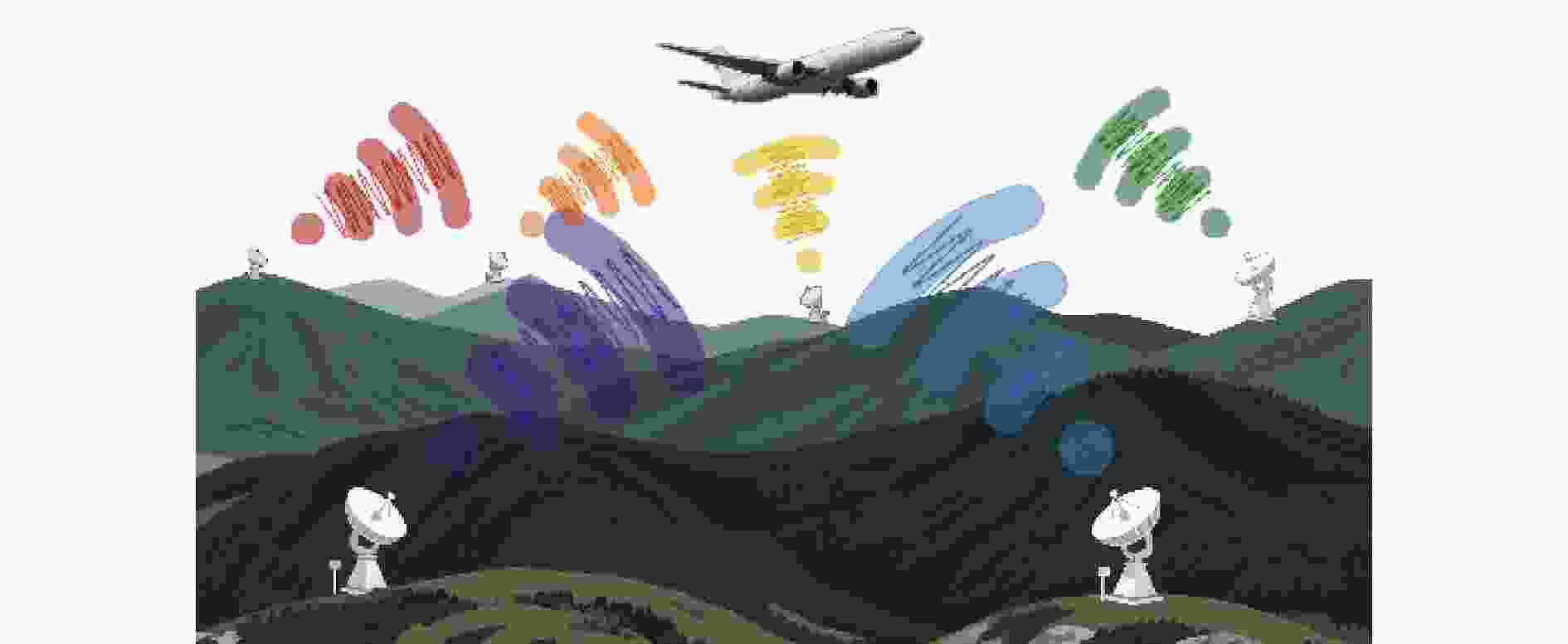
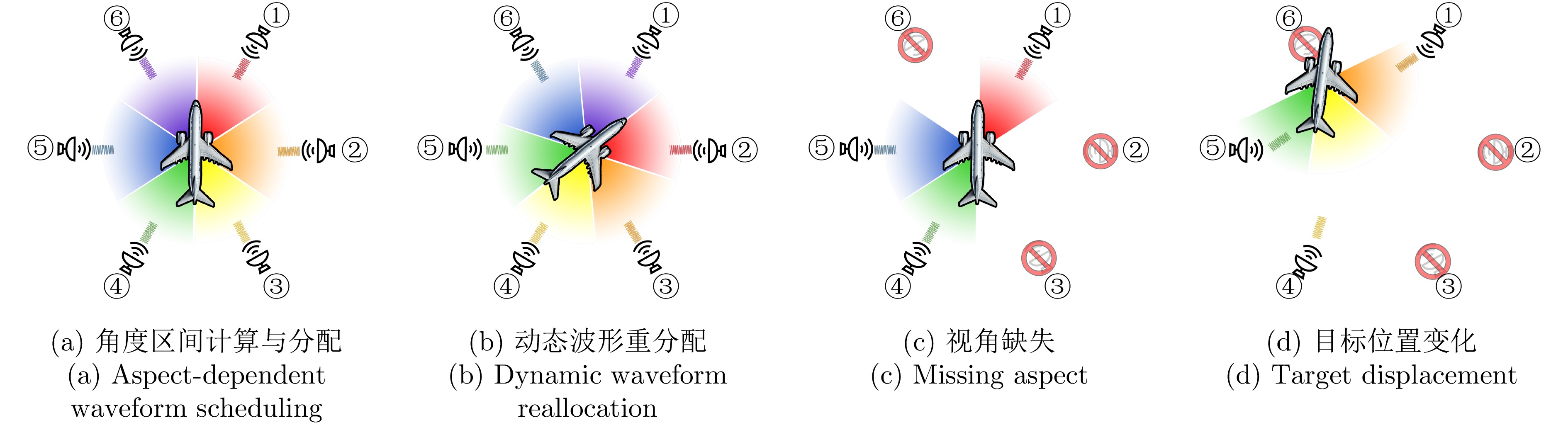
图 1 分布式雷达多波形协同识别示意图
Figure 1. Illustration of distributed radar recognition via multi-waveform cooperation
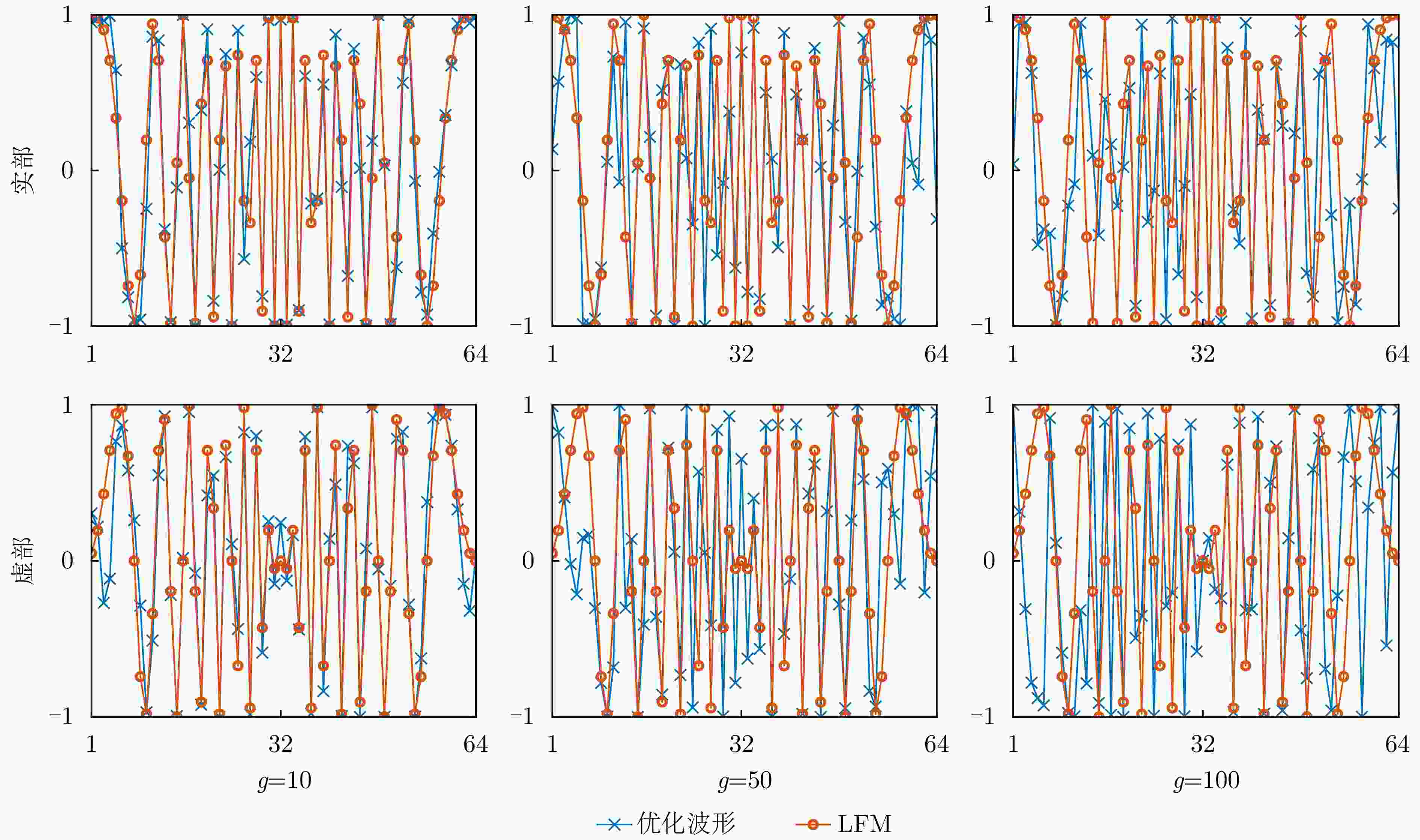
图 8 不同学习率倍率下LFM与优化波形对比
Figure 8. Comparison between LFM and the optimized waveform under different learning rate multiplier
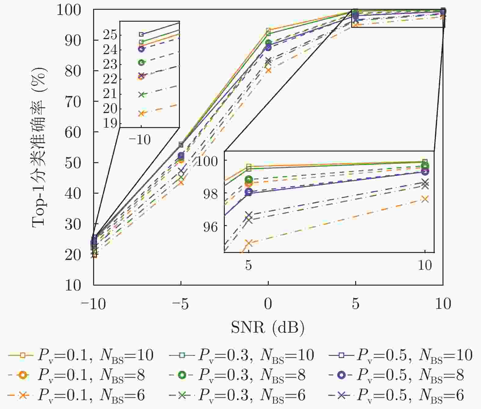
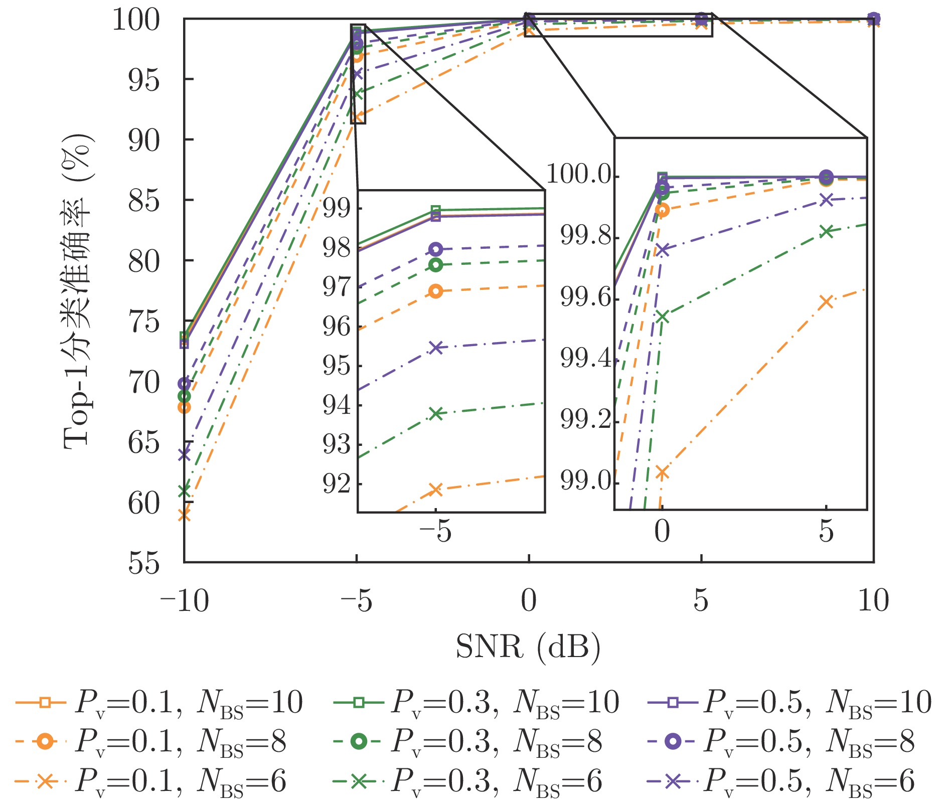
图 10 民用车辆TIR数据集不同基站数量下时域波形设计分类准确率
Figure 10. Classification accuracy under different numbers of base stations for the time-domain waveform design on the civilian vehicle TIR dataset
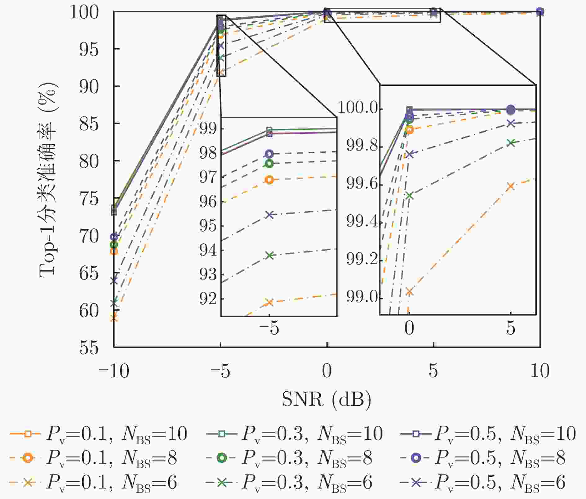
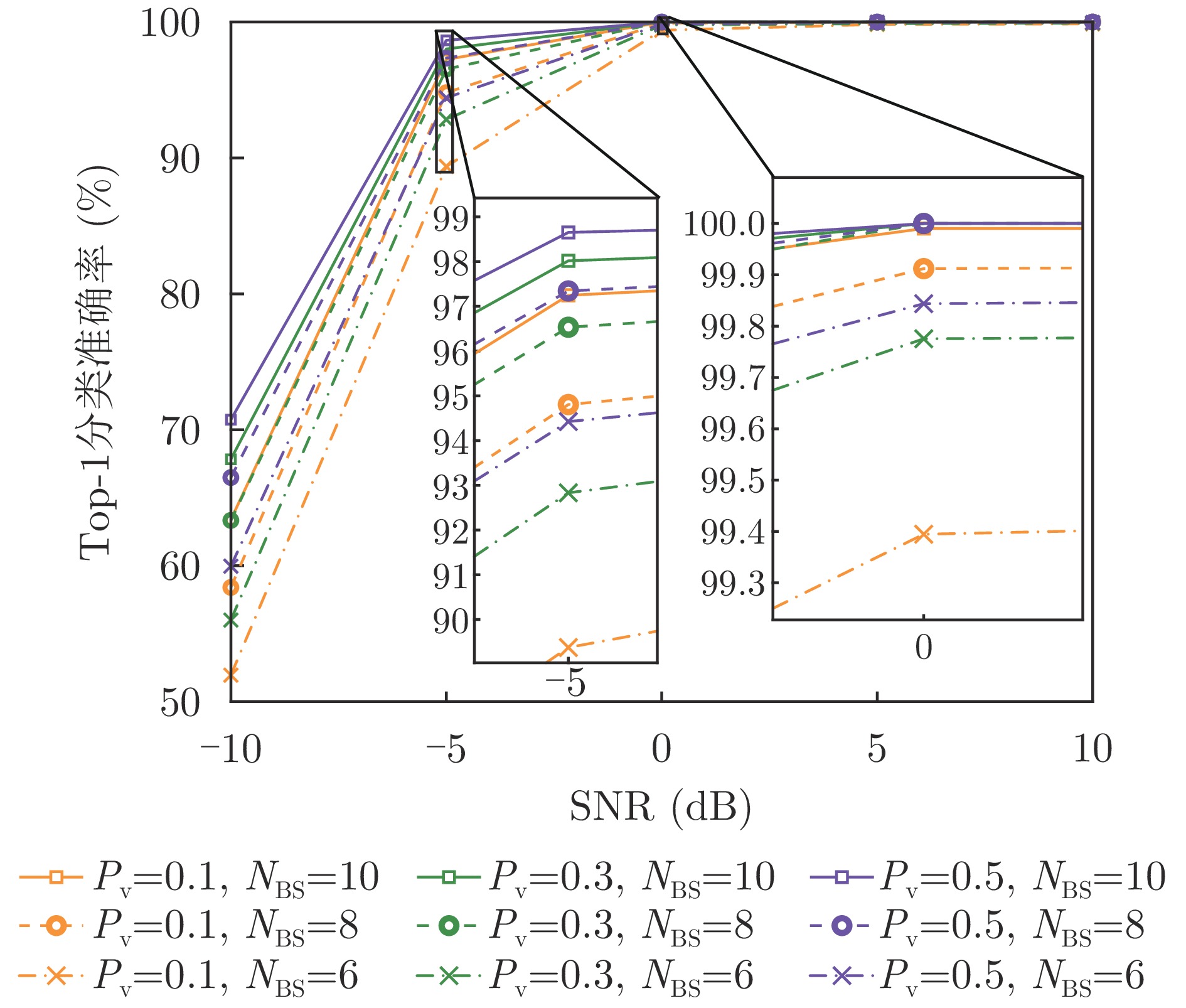
图 11 民用车辆TFR数据集不同基站数量下频域波形设计分类准确率
Figure 11. Classification accuracy under different numbers of base stations for the frequency-domain waveform design on the civilian vehicle TFR dataset
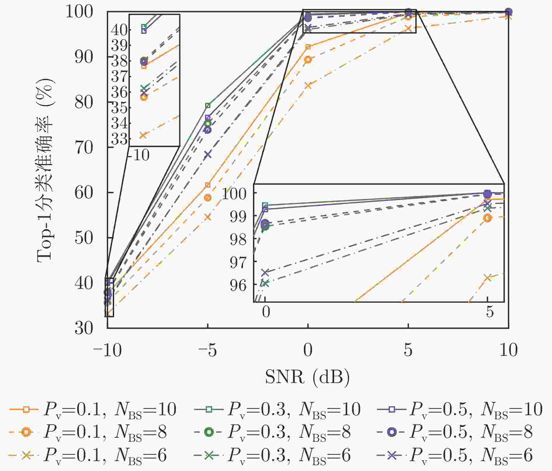
图 12 电磁仿真TIR数据集不同基站数量下时域波形设计分类准确率
Figure 12. Classification accuracy under different numbers of base stations for the time-domain waveform design on the electromagnetic simulation TIR dataset
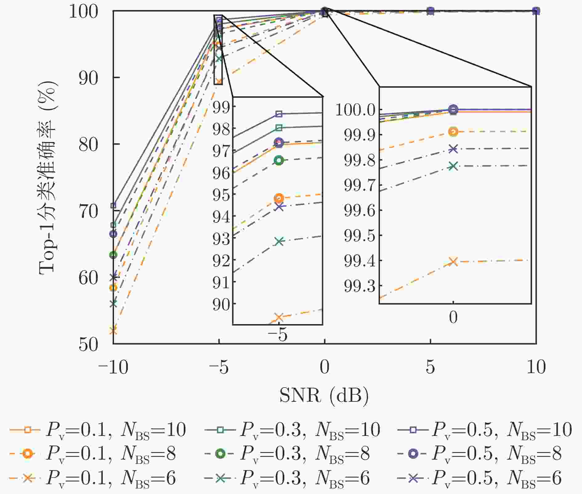
图 13 电磁仿真TFR数据集不同基站数量下频域波形设计分类准确率
Figure 13. Classification accuracy under different numbers of base stations for the frequency-domain waveform design on the electromagnetic simulation TFR dataset
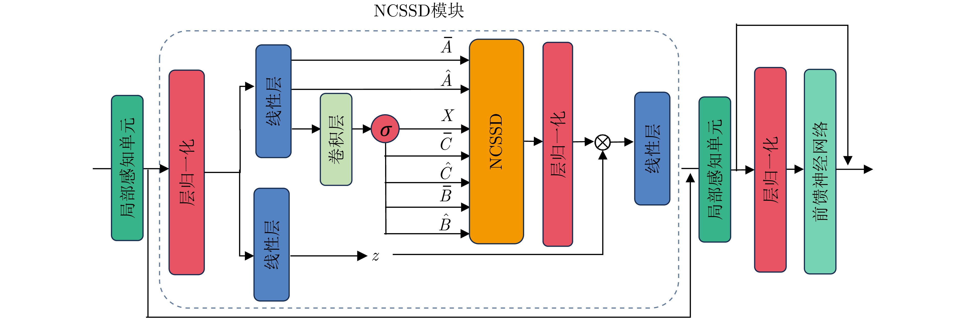
1 NCSSD模块核心组件
1. Core components of the NCSSD block
输入:序列$ {\boldsymbol{S}}_{\mathrm{in}} $,参数$ {{\varDelta }}_{\text{in}} $, $ {\hat{A}}_{\mathrm{in}} $和$ {\bar{A}}_{\mathrm{in}} $ #$ {\boldsymbol{S}}_{\mathrm{in}}\in {\mathbb{R}}^{C\times L}\text{,}\;{{\varDelta }}_{\text{in}},\;{\hat{A}}_{\mathrm{in}}\mathbf{,}\;{\bar{A}}_{\mathrm{in}}\in {\mathbb{R}}^{H} $ 输出:序列$ {\boldsymbol{S}}_{\text{out}} $ #$ {\boldsymbol{S}}_{\text{out}}\in {\mathbb{R}}^{C\times L} $ 步骤1:构造SSM所需变量 1:$ \boldsymbol{S}_{\mathrm{in}}^{\prime}\leftarrow \mathrm{Norm}\left({\boldsymbol{S}}_{\mathrm{in}}\right) $ #$ \boldsymbol{S}_{\mathrm{in}}^{\prime}\in {\mathbb{R}}^{C\times L} $ 2:$ \boldsymbol{Z}\leftarrow {\text{Linear}}^{\boldsymbol{Z}}\left(\boldsymbol{S}_{\text{in}}^{\prime}\right) $ #$ \boldsymbol{Z}\in {\mathbb{R}}^{2C\times L} $ 3:$ {{\boldsymbol{\varDelta}} }^{\prime}\leftarrow {\text{Linear}}^{{{{\boldsymbol{\varDelta}} }^{\prime}}}\left(\boldsymbol{S}_{\text{in}}^{\prime}\right) $ #$ {{\boldsymbol{\varDelta}} }^{\prime}\in {\mathbb{R}}^{H\times L} $ 4:$ \boldsymbol{X},{\hat{{\boldsymbol{B}}} }^{\prime},{\bar{{\boldsymbol{B}}} }^{\prime},\hat{{\boldsymbol{C}}} ,\bar{{\boldsymbol{C}}} \leftarrow \mathrm{SiLU}\left(\mathrm{Conv}1\mathrm{d}\left(\mathrm{Linear}\left(\boldsymbol{S}_{\text{in}}^{\prime}\right)\right)\right) $ #Conv1d为核为3的深度卷积 #$ \boldsymbol{X}\in {\mathbb{R}}^{H\times {2C}/{H}\times L} $, $ {\hat{{\boldsymbol{B}}} }^{\prime},{\bar{{\boldsymbol{B}}} }^{\prime}\in {\mathbb{R}}^{1\times D\times L} $, $ \hat{{\boldsymbol{C}}} ,\bar{{\boldsymbol{C}}} $$ \in {\mathbb{R}}^{1\times D\times L} $ 5:$ {\boldsymbol{\varDelta}} \leftarrow \mathrm{Softplus}\left({{\boldsymbol{\varDelta}} }^{\prime}+{{\varDelta }}_{\text{in}}\right) $ #$ {\boldsymbol{\varDelta}} \in {\mathbb{R}}^{H\times L} $ 6:$ \hat{\boldsymbol{A}}\mathbf{,}\;\bar{\boldsymbol{A}}\leftarrow {\boldsymbol{\varDelta}} \times {\hat{A}}_{\mathrm{in}},{\boldsymbol{\varDelta}} \times {\bar{{\boldsymbol{A}}}}_{\mathrm{in}} $ #$ \hat{\boldsymbol{A}},\bar{\boldsymbol{A}}\in {\mathbb{R}}^{H\times L} $ 7:$ \hat{\boldsymbol{B}},\bar{\boldsymbol{B}}\leftarrow {\boldsymbol{\varDelta}} \times {\hat{{\boldsymbol{B}}} }^{\prime},{\boldsymbol{\varDelta}} \times {\bar{{\boldsymbol{B}}} }^{\prime} $ #$ \hat{\boldsymbol{B}},\bar{\boldsymbol{B}}\in {\mathbb{R}}^{H\times D\times L} $ 步骤2:使用NCSSD实现非因果的SSM计算(见算法2) 8:$ \boldsymbol{Y}\leftarrow {\mathrm{SSM}}_{\hat{\boldsymbol{A}},\bar{\boldsymbol{A}},\hat{\boldsymbol{B}},\bar{\boldsymbol{B}},\hat{{\boldsymbol{C}}} ,\bar{{\boldsymbol{C}}} }(\boldsymbol{X}) $ #$ \boldsymbol{Y}\in {\mathbb{R}}^{2C\times L} $ 步骤3:计算输出序列$ {\boldsymbol{S}}_{\text{out}} $ 9:$ {\boldsymbol{Y}}_{\text{g}}\leftarrow \mathrm{Norm}(\boldsymbol{Y})\odot \boldsymbol{Z} $ #$ {\boldsymbol{Y}}_{\text{g}}\in {\mathbb{R}}^{2C\times L} $ 10:$ {\boldsymbol{S}}_{\text{out}}\leftarrow {\text{Linear}}^{{{\boldsymbol{S}}_{\text{out}}}}\left({\boldsymbol{Y}}_{\text{g}}\right) $ #$ {\boldsymbol{S}}_{\text{out}}\in {\mathbb{R}}^{C\times L} $  下载: 导出CSV
2 基于结构化矩阵的NCSSD高效算法
2. An Efficient algorithm based on structured matrices
输入:张量$ \boldsymbol{X} $, $ \bar{\boldsymbol{A}} $, $ \hat{\boldsymbol{A}} $, $ \bar{\boldsymbol{B}} $, $ \hat{\boldsymbol{B}} $, $ \bar{\boldsymbol{C}} $, $ \hat{\boldsymbol{C}} $子块大小l 输出:张量 $ \boldsymbol{Y} $ 初始化:将张量$ \boldsymbol{X} $, $ \bar{\boldsymbol{A}} $, $ \hat{\boldsymbol{A}} $, $ \bar{\boldsymbol{B}} $, $ \hat{\boldsymbol{B}} $, $ \bar{\boldsymbol{C}} $, $ \hat{\boldsymbol{C}} $按子块大小l重新排布 调整$ \bar{\boldsymbol{A}} $和$ \hat{\boldsymbol{A}} $维度:$ (b,c,l,h)\rightarrow (b,h,c,l) $ 计算累积和:$ {\hat{\boldsymbol{A}}}_{\text{cum}}=\mathrm{cumsum}(\hat{\boldsymbol{A}},\dim =-1) $, $ {\bar{\boldsymbol{A}}}_{\text{cum}}=\mathrm{cumsum}(\bar{\boldsymbol{A}},\dim =-1) $ 步骤1:计算对角块内输出 $ \bar{\boldsymbol{L}}=\exp (\mathrm{segsum}(\mathrm{pad}(\bar{\boldsymbol{A}}[\colon ,\colon ,\colon ,\colon -1],(1,0)))) $,$ \hat{\boldsymbol{L}}=\exp (\mathrm{segsum}(\hat{\boldsymbol{A}})) $ $ {\bar{\boldsymbol{Y}}}_{\text{diag}}=\mathrm{einsum}(bclhn,bcshn,bhcsl,bcshp\rightarrow bclhp,\bar{\boldsymbol{C}},\bar{\boldsymbol{B}},\bar{\boldsymbol{L}},\boldsymbol{X}) $ $ {\hat{\boldsymbol{Y}}}_{\text{diag}}=\mathrm{einsum}(bclhn,bcshn,bhcsl,bcshp\rightarrow bclhp,\hat{\boldsymbol{C}},\hat{\boldsymbol{B}},\hat{\boldsymbol{L}},\boldsymbol{X}) $ $ {\boldsymbol{Y}}_{\text{diag}}={\bar{\boldsymbol{Y}}}_{\text{diag}}+{\hat{\boldsymbol{Y}}}_{\text{diag}} $ 步骤2:计算每个内部块的状态 $ \widehat{\bf{d}\bf{e}\bf{c}}=\exp \left({\hat{\boldsymbol{A}}}_{\text{cum}}[\colon ,\colon ,\colon ,-1\colon ]-{\hat{\boldsymbol{A}}}_{\text{cum}}\right) $ $ \bar{\bf{d}\bf{e}\bf{c}}=\exp \left(\mathrm{pad}\left({\bar{\boldsymbol{A}}}_{\text{cum}}[\colon ,\colon ,\colon ,\colon -1],(1,0)\right)\right) $ $ \widehat{\bf{s}\bf{t}\bf{s}}=\mathrm{einsum}(bclhn,bhcl,bclhp\rightarrow bchpn,\hat{\boldsymbol{B}},\widehat{\bf{d}\bf{e}\bf{c}},\boldsymbol{X}) $ $ \bar{\bf{s}\bf{t}\bf{s}}=\mathrm{einsum}(bclhn,bhcl,bclhp\rightarrow bchpn,\bar{\boldsymbol{B}},\bar{\bf{d}\bf{e}\bf{c}},\boldsymbol{X}) $ 步骤3:计算块间递归 $ \widehat{\bf{s}\bf{t}\bf{s}}=\mathrm{concat}\left(\left[\bf{i}\bf{n}\bf{i}\bf{t}\_ \bf{s}\bf{t}\bf{s},\widehat{\bf{s}\bf{t}\bf{s}}\right],\dim =1\right) $ $ \bar{\bf{s}\bf{t}\bf{s}}=\mathrm{concat}\left(\left[\bf{i}\bf{n}\bf{i}\bf{t}\_ \bf{s}\bf{t}\bf{s},\bar{\bf{s}\bf{t}\bf{s}}\right],\dim =1\right) $$ (b,c,l,h,p)\rightarrow (b,c*l,h*p) $ $ {\widehat{\bf{d}\bf{e}\bf{c}}}_{\text{chunk}}=\exp \left(\mathrm{segsum}\left(\mathrm{pad}\left({\hat{\boldsymbol{A}}}_{\text{cum}}[\colon ,\colon ,\colon ,-1],(1,0)\right)\right)\right) $ $ {\bar{\bf{d}\bf{e}\bf{c}}}_{\text{chunk}}=\exp \left(\mathrm{segsum}\left(\mathrm{pad}\left({\bar{\boldsymbol{A}}}_{\text{cum}}[\colon ,\colon ,\colon ,-1],(1,0)\right)\right)\right) $ $ {\bf{n}\bf{e}\bf{w}}\_ {\bf{s}\bf{t}\bf{s}}\text{=}\mathrm{einsum}\left(bhzc,bchpn\rightarrow bzhpn,{\widehat{\bf{d}\bf{e}\bf{c}}}_{\text{chunk}},\widehat{\bf{s}\bf{t}\bf{s}}\right) $ $ \widehat{\bf{s}\bf{t}\bf{s}}=\bf{n}\bf{e}\bf{w}\_ \bf{s}\bf{t}\bf{s}[\colon ,\colon -1] $ $ \bar{\bf{s}\bf{t}\bf{s}}=\mathrm{einsum}\left(bhcz,bchpn\rightarrow bzhpn,{\bar{\bf{d}\bf{e}\bf{c}}}_{\text{chunk}},\bar{\bf{s}\bf{t}\bf{s}}\right) $ 步骤4:计算块状态到输出的转换 $ {\widehat{\bf{s}\bf{t}\bf{s}}}_{{{\mathrm{dec}}\_{\mathrm{out}}}}=\exp \left({\hat{\boldsymbol{A}}}_{\text{cum}}\right) $ $ {\bar{\bf{s}\bf{t}\bf{s}}}_{{{\mathrm{dec}}\_{\mathrm{out}}}}=\exp \left({\bar{\boldsymbol{A}}}_{\text{cum}}[\colon ,\colon ,\colon ,-1\colon ]-\mathrm{pad}\left({\bar{\boldsymbol{A}}}_{\text{cum}}[\colon ,\colon ,\colon ,\colon -1],(1,0)\right)\right) $ $ {\hat{\boldsymbol{Y}}}_{\text{off}}=\mathrm{einsum}\left(\hat{\boldsymbol{C}},\widehat{\bf{s}\bf{t}\bf{s}},{\widehat{\bf{s}\bf{t}\bf{s}}}_{{{\mathrm{dec}}\_{\mathrm{out}}}}\right) $ $ {\bar{\boldsymbol{Y}}}_{\text{off}}=\mathrm{einsum}\left(\bar{\boldsymbol{C}},\bar{\bf{s}\bf{t}\bf{s}}\mathbf{,}{\bar{\bf{s}\bf{t}\bf{s}}}_{{{\mathrm{dec}}\_{\mathrm{out}}}}\right) $ $ \boldsymbol{Y}={\boldsymbol{Y}}_{\text{diag}}+{\hat{\boldsymbol{Y}}}_{\text{off}}+{\bar{\boldsymbol{Y}}}_{\text{off}} $
下载: 导出CSV
表 1 网络超参数设置
Table 1. Network hyperparameter settings
参数 电磁仿真数据集
网络$ {{C}}_{\boldsymbol{\phi }1} $民用车辆数据集
网络$ {{C}}_{\boldsymbol{\phi }2} $堆叠数量$ {N}_{1},{N}_{2},{N}_{3} $ 1, 1, 2 2, 1, 2 多头数量$ {H}_{1},{H}_{2},{H}_{3} $ 1, 2, 4 2, 8, 8 通道数$ {C}_{1},{C}_{2} $ 16, 64 16, 128 训练轮数 40 80 峰值学习率(余弦退火) $ 1\times {10}^{-3} $ $ 3\times {10}^{-4} $
下载: 导出CSV
表 2 模型各阶段参数量与计算量
Table 2. Parameter count and FLOPs for each stage of the model
参数 DRWC (NCSSD) DRWC (SSD) 电磁仿真 民用车辆 电磁仿真 民用车辆 特征提取参数量 16.71 K 23.38 K 15.43 K 20.81 K 单视角特征提取FLOPs 1.31 M 3.10 M 0.81 M 1.97 M 融合推理参数量 1.40 M 5.31 M 1.36 M 5.23 M 融合推理FLOPs 23.24 M 114.88 M 20.38 M 101.67 M 总参数量 1.42 M 5.33 M 1.38 M 5.25 M 总FLOPs 37.14 M 147.00 M 29.32 M 122.48 M
下载: 导出CSV
表 3 民用车辆数据集不同信噪比下各网络分类准确率(%)
Table 3. Classification accuracy of different networks across various SNRs on the civilian vehicle dataset (%)
网络 TIR数据集 TFR数据集 –10 dB –5 dB 0 dB 5 dB 10 dB –10 dB –5 dB 0 dB 5 dB 10 dB SV-RWC 12.36 16.95 27.82 42.82 51.99 18.24 38.13 67.14 83.05 88.32 DRWC-S 21.46 39.53 67.94 85.95 91.74 54.81 92.08 99.41 99.89 99.91 DRWC-P 24.67 53.11 87.37 97.69 99.19 71.31 98.76 100.00 100.00 100.00 SAM 23.58 52.59 86.10 97.43 98.88 66.62 97.46 99.98 100.00 100.00 SSD 23.93 53.86 87.03 97.65 99.30 70.21 98.50 99.99 100.00 100.00 DRWC-SP 25.05 55.66 88.25 97.97 99.29 73.05 98.79 100.00 100.00 100.00 注:表中加粗数值表示各信噪比条件下各网络的最高准确率。
下载: 导出CSV
表 4 电磁仿真数据集不同信噪比下各网络分类准确率(%)
Table 4. Classification accuracy of different networks across various SNRs on the electromagnetic simulation dataset (%)
网络 TIR数据集 TFR数据集 –10 dB –5 dB 0 dB 5 dB 10 dB –10 dB –5 dB 0 dB 5 dB 10 dB SV-RWC 22.47 31.77 62.88 90.00 96.43 28.13 52.29 89.21 99.21 99.87 DRWC-S 33.80 58.78 92.22 99.55 99.94 53.33 92.39 99.90 100.00 100.00 DRWC-P 38.64 76.41 99.13 99.99 100.00 69.39 98.52 100.00 100.00 100.00 SAM 37.29 75.31 99.24 100.00 100.00 67.28 98.13 100.00 100.00 100.00 SSD 38.73 76.47 99.14 99.99 100.00 68.68 98.41 100.00 100.00 100.00 DRWC-SP 39.91 76.61 99.28 100.00 100.00 70.74 98.65 100.00 100.00 100.00 注:表中加粗数值表示各信噪比条件下各网络的最高准确率。
下载: 导出CSV
表 5 民用车辆TIR数据集不同波形与波形数量在各信噪比条件下分类准确率(%)
Table 5. Classification accuracy vs. waveform type, number of waveforms, and SNR on the civilian vehicle TIR dataset (%)
网络设置 –10 dB –5 dB 0 dB 5 dB 10 dB P4+$ {{C}}_{\boldsymbol{\phi }1} $ 25.21 54.78 86.35 97.45 99.01 LFM+$ {{C}}_{\boldsymbol{\phi }1} $ 24.36 53.79 84.91 96.74 98.71 时域UniWGM+$ {{C}}_{\boldsymbol{\phi }1} $, $ {N}_{\text{w}}=1 $ 25.40 55.52 86.55 97.63 99.12 时域WGM+$ {{C}}_{\boldsymbol{\phi }1} $, $ {N}_{\text{w}}=1 $ 26.98 57.28 88.04 97.86 99.25 时域WGM+$ {{C}}_{\boldsymbol{\phi }1} $, $ {N}_{\text{w}}=8 $ 33.60 68.94 93.56 98.80 99.43 时域 WGM+$ {{C}}_{\boldsymbol{\phi }1} $, $ {N}_{\text{w}}=16 $ 34.52 70.91 94.57 99.01 99.54 注:表中加粗数值表示各信噪比下,单波形和多波形设置下各网络的最高准确率。
下载: 导出CSV
表 6 民用车辆TFR数据集不同波形与波形数量在各信噪比条件下分类准确率(%)
Table 6. Classification accuracy vs. waveform type, number of waveforms, and SNR on the civilian vehicle TFR dataset (%)
网络设置 –10 dB –5 dB 0 dB 5 dB 10 dB P4+$ {{C}}_{\boldsymbol{\phi }1} $ 70.91 98.51 99.99 100.00 100.00 LFM+$ {{C}}_{\boldsymbol{\phi }1} $ 69.96 98.41 99.99 100.00 100.00 频域UniWGM+$ {{C}}_{\boldsymbol{\phi }1} $, $ {N}_{\text{w}}=1 $ 70.99 98.54 99.99 100.00 100.00 频域WGM+$ {{C}}_{\boldsymbol{\phi }1} $, $ {N}_{\text{w}}=1 $ 71.14 98.58 100.00 100.00 100.00 频域WGM+$ {{C}}_{\boldsymbol{\phi }1} $, $ {N}_{\text{w}}=8 $ 73.20 98.91 100.00 100.00 100.00 频域 WGM+$ {{C}}_{\boldsymbol{\phi }1} $, $ {N}_{\text{w}}=16 $ 73.47 98.98 100.00 100.00 100.00 注:表中加粗数值表示各信噪比下,单波形和多波形设置下各网络的最高准确率。
下载: 导出CSV
表 7 电磁仿真TIR数据集不同波形与波形数量在各信噪比条件下分类准确率(%)
Table 7. Classification accuracy vs. waveform type, number of waveforms, and SNR on the electromagnetic simulation TIR dataset (%)
网络设置 –10 dB –5 dB 0 dB 5 dB 10 dB P4+$ {{C}}_{\boldsymbol{\phi }2} $ 39.21 76.90 98.93 100.00 100.00 LFM+$ {{C}}_{\boldsymbol{\phi }2} $ 40.14 77.21 98.90 100.00 100.00 时域UniWGM+$ {{C}}_{\boldsymbol{\phi }2} $, $ {N}_{\text{w}}=1 $ 40.51 77.43 98.96 99.99 100.00 时域WGM+$ {{C}}_{\boldsymbol{\phi }2} $, $ {N}_{\text{w}}=1 $ 41.11 77.69 99.02 99.97 100.00 时域WGM+$ {{C}}_{\boldsymbol{\phi }2} $, $ {N}_{\text{w}}=8 $ 41.94 76.43 99.07 100.00 100.00 时域 WGM+$ {{C}}_{\boldsymbol{\phi }2} $, $ {N}_{\text{w}}=16 $ 42.97 79.02 99.33 100.00 100.00 注:表中加粗数值表示各信噪比下,单波形和多波形设置下各网络的最高准确率。
下载: 导出CSV
表 8 电磁仿真TFR数据集不同波形与波形数量在各信噪比条件下分类准确率(%)
Table 8. Classification accuracy vs. waveform type, number of waveforms, and SNR on the electromagnetic simulation TFR dataset (%)
网络设置 –10 dB –5 dB 0 dB 5 dB 10 dB P4+$ {{C}}_{\boldsymbol{\phi }2} $ 71.55 98.60 100.00 100.00 100.00 LFM+$ {{C}}_{\boldsymbol{\phi }2} $ 69.59 98.33 100.00 100.00 100.00 频域UniWGM+$ {{C}}_{\boldsymbol{\phi }2} $, $ {N}_{\text{w}}=1 $ 71.89 98.61 100.00 100.00 100.00 频域WGM+$ {{C}}_{\boldsymbol{\phi }2} $, $ {N}_{\text{w}}=1 $ 72.15 98.64 100.00 100.00 100.00 频域WGM+$ {{C}}_{\boldsymbol{\phi }2} $, $ {N}_{\text{w}}=8 $ 72.69 98.79 100.00 100.00 100.00 频域 WGM+$ {{C}}_{\boldsymbol{\phi }2} $, $ {N}_{\text{w}}=16 $ 73.17 98.80 100.00 100.00 100.00 注:表中加粗数值表示各信噪比下,单波形和多波形设置下各网络的最高准确率。
下载: 导出CSV
表 9 各信噪比条件下时频域处理网络分类准确率(%)
Table 9. Classification accuracy for time-domain and frequency-domain processing networks under different SNRs (%)
网络 –10 dB –5 dB 0 dB 5 dB 10 dB T-DRWC-S 22.96 38.45 81.92 97.79 98.91 T-DRWC-P 28.79 54.37 94.54 99.99 100.00 T-DRWC 29.58 55.84 95.65 99.99 100.00 F-DRWC-S 23.82 38.69 82.80 97.84 98.69 F-DRWC-P 26.32 47.98 90.30 99.88 100.00 F-DRWC 27.42 49.86 92.56 99.85 100.00 注:表中加粗数值表示各信噪比下时域网络与频域网络最高分类准确率。
下载: 导出CSV
-
[1] HE Hao, LI Jian, and STOICA P. Waveform Design for Active Sensing Systems: A Computational Approach[M]. Cambridge: Cambridge University Press, 2012. doi: 10.1017/CBO9781139095174. [2] BLUNT S D and MOKOLE E L. Overview of radar waveform diversity[J]. IEEE Aerospace and Electronic Systems Magazine, 2016, 31(11): 2–42. doi: 10.1109/MAES.2016.160071. [3] WANG Jiahang, LIANG Junli, CHENG Zhiwei, et al. Radar waveform design based on target pattern separability via fractional programming[J]. IEEE Transactions on Signal Processing, 2024, 72: 2543–2559. doi: 10.1109/TSP.2024.3387335. [4] HU Jinfeng, WEI Zhiyong, LI Yuzhi, et al. Designing unimodular waveform(s) for MIMO radar by deep learning method[J]. IEEE Transactions on Aerospace and Electronic Systems, 2021, 57(2): 1184–1196. doi: 10.1109/TAES.2020.3037406. [5] ZHONG Kai, ZHANG Weijian, ZHANG Qiping, et al. MIMO radar waveform design via deep learning[C]. The IEEE Radar Conference, Atlanta, USA, 2021: 1–5. doi: 10.1109/RadarConf2147009.2021.9455163. [6] PEI Yaya, HU Jinfeng, ZHONG Kai, et al. MIMO radar waveform optimization by deep learning method[C]. The IEEE International Geoscience and Remote Sensing Symposium, Kuala Lumpur, Malaysia, 2022: 811–814. doi: 10.1109/IGARSS46834.2022.9884371. [7] XIA M, GONG W R, and YANG L C. A novel waveform optimization method for orthogonal-frequency multiple-input multiple-output radar based on dual-channel neural networks[J]. Sensors, 2024, 24(17): 5471. doi: 10.3390/s24175471. [8] YAN Bo, PAOLINI E, XU Luping, et al. A target detection and tracking method for multiple radar systems[J]. IEEE Transactions on Geoscience and Remote Sensing, 2022, 60: 5114721. doi: 10.1109/TGRS.2022.3183387. [9] LU Jing, ZHOU Shenghua, PENG Xiaojun, et al. Distributed radar multiframe detection with local censored observations[J]. IEEE Transactions on Aerospace and Electronic Systems, 2024, 60(6): 9006–9028. doi: 10.1109/TAES.2024.3438103. [10] CAO Xiaomao, YI Jianxin, GONG Ziping, et al. Automatic target recognition based on RCS and angular diversity for multistatic passive radar[J]. IEEE Transactions on Aerospace and Electronic Systems, 2022, 58(5): 4226–4240. doi: 10.1109/TAES.2022.3159295. [11] PU Weiming, LIANG Zhennan, WU Jianxin, et al. Joint generalized inner product method for main lobe jamming suppression in distributed array radar[J]. IEEE Transactions on Aerospace and Electronic Systems, 2023, 59(5): 6940–6953. doi: 10.1109/TAES.2023.3280892. [12] PU Weiming, ZHENG Ziming, TIAN Dezhi, et al. Velocity estimation of DRFM jamming source based on Doppler differences in distributed array radar[C]. The IET International Radar Conference, Chongqing, China, 2023: 387–392. doi: 10.1049/icp.2024.1110. [13] LINGADEVARU P, PARDHASARADHI B, and SRIHARI P. Sequential fusion based approach for estimating range gate pull-off parameter in a networked radar system: An ECCM algorithm[J]. IEEE Access, 2022, 10: 70902–70918. doi: 10.1109/ACCESS.2022.3185240. [14] BELL M R. Information theory and radar waveform design[J]. IEEE Transactions on Information Theory, 1993, 39(5): 1578–1597. doi: 10.1109/18.259642. [15] GARREN D A, OSBORN M K, ODOM A C, et al. Enhanced target detection and identification via optimised radar transmission pulse shape[J]. IEE Proceedings - Radar, Sonar and Navigation, 2001, 148(3): 130–138. doi: 10.1049/ip-rsn:20010324. [16] GARREN D A, OSBORN M K, ODOM A C, et al. Optimal transmission pulse shape for detection and identification with uncertain target aspect[C]. The IEEE Radar Conference, Atlanta, USA, 2001: 123–128. doi: 10.1109/NRC.2001.922963. [17] GARREN D A, ODOM A C, OSBORN M K, et al. Full-polarization matched-illumination for target detection and identification[J]. IEEE Transactions on Aerospace and Electronic Systems, 2002, 38(3): 824–837. doi: 10.1109/TAES.2002.1039402. [18] ROMERO R A, BAE J, and GOODMAN N A. Theory and application of SNR and mutual information matched illumination waveforms[J]. IEEE Transactions on Aerospace and Electronic Systems, 2011, 47(2): 912–927. doi: 10.1109/TAES.2011.5751234. [19] ALSHIRAH S Z, GISHKORI S, and MULGREW B. Frequency-based optimal radar waveform design for classification performance maximization using multiclass fisher analysis[J]. IEEE Transactions on Geoscience and Remote Sensing, 2021, 59(4): 3010–3021. doi: 10.1109/TGRS.2020.3008562. [20] DU Lan, LIU Hongwei, and BAO Zheng. Radar HRRP statistical recognition: Parametric model and model selection[J]. IEEE Transactions on Signal Processing, 2008, 56(5): 1931–1944. doi: 10.1109/TSP.2007.912283. [21] TAN Q J O, ROMERO R A, and JENN D C. Target recognition with adaptive waveforms in cognitive radar using practical target RCS responses[C]. The IEEE Radar Conference, Oklahoma City, USA, 2018: 0606–0611. doi: 10.1109/RADAR.2018.8378628. [22] WU Zhongjie, WANG Chenxu, LI Yingchun, et al. Extended target estimation and recognition based on multimodel approach and waveform diversity for cognitive radar[J]. IEEE Transactions on Geoscience and Remote Sensing, 2022, 60: 5101014. doi: 10.1109/TGRS.2021.3065335. [23] GOYAL A and BENGIO Y. Inductive biases for deep learning of higher-level cognition[EB/OL]. https://doi.org/10.48550/arXiv.2011.15091, 2020. [24] BHALLA R, LING H, MOORE J, et al. 3D scattering center representation of complex targets using the shooting and bouncing ray technique: A review[J]. IEEE Antennas and Propagation Magazine, 1998, 40(5): 30–39. doi: 10.1109/74.735963. [25] DING Baiyuan and WEN Gongjian. Target reconstruction based ON 3-D scattering center model for robust SAR ATR[J]. IEEE Transactions on Geoscience and Remote Sensing, 2018, 56(7): 3772–3785. doi: 10.1109/TGRS.2018.2810181. [26] LEI Wei, ZHANG Yue, and CHEN Zengping. A real-time fine echo generation method of extended false target with radially high-speed moving[J]. IET Radar, Sonar & Navigation, 2023, 17(2): 312–325. doi: 10.1049/rsn2.12342. [27] LIANG Junli, SO H C, LI Jian, et al. Unimodular sequence design based on alternating direction method of multipliers[J]. IEEE Transactions on Signal Processing, 2016, 64(20): 5367–5381. doi: 10.1109/TSP.2016.2597123. [28] VASWANI A, SHAZEER N, PARMAR N, et al. Attention is all you need[C]. The 31st International Conference on Neural Information Processing Systems, Long Beach, USA, 2017: 6000–6010. [29] FAN Wen, LIANG Junli, CHEN Zihao, et al. Spectrally compatible aperiodic sequence set design with low cross- and auto-correlation PSL[J]. Signal Processing, 2021, 183: 107960. doi: 10.1016/j.sigpro.2020.107960. [30] GU A and DAO T. Mamba: Linear-time sequence modeling with selective state spaces[EB/OL]. https://doi.org/10.48550/arXiv.2312.00752, 2023. [31] GU A, DAO T, EEMON S, et al. HiPPO: Recurrent memory with optimal polynomial projections[EB/OL]. https://doi.org/10.48550/arXiv.2008.07669, 2020. [32] GU A, GOEL K, and RÉ C. Efficiently modeling long sequences with structured state spaces[EB/OL]. https://doi.org/10.48550/arXiv.2111.00396, 2021. [33] GU A, JOHNSON I, GOEL K, et al. Combining recurrent, convolutional, and continuous-time models with linear state-space layers[C]. The 35th International Conference on Neural Information Processing System, Vancouver, Canada, 2021: 44. [34] DAO T and GU A. Transformers are SSMs: Generalized models and efficient algorithms through structured state space duality[EB/OL]. https://doi.org/10.48550/arXiv.2405.21060, 2024. [35] GUO Jianyuan, HAN Kai, WU Han, et al. CMT: Convolutional neural networks meet vision transformers[EB/OL]. https://doi.org/10.48550/arXiv.2107.06263, 2021. [36] DOSOVITSKIY A, BEYER L, KOLESNIKOV A, et al. An image is worth 16x16 words: Transformers for image recognition at scale[C]. The 9th International Conference on Learning Representations, 2021. [37] SHI Yuheng, DONG Minjing, LI Mingjia, et al. VSSD: Vision Mamba with non-causal state space duality[EB/OL]. https://doi.org/10.48550/arXiv.2407.18559, 2024. [38] HAN Dongchen, WANG Ziyi, XIA Zhuofan, et al. Demystify Mamba in vision: A linear attention perspective[EB/OL]. https://doi.org/10.48550/arXiv.2405.16605, 2024. [39] ALTAIR. Feko (2023) [Electromagnetic simulation software][CP/OL]. https://www.altair.com/feko, 2023. [40] SDMS. Civilian vehicle data dome overview[DS/OL]. https://www.sdms.afrl.af.mil/index.php?collection=cv_dome, 2025. [41] HE Kaiming, ZHANG Xiangyu, REN Shaoqing, et al. Deep residual learning for image recognition[C]. The IEEE Conference on Computer Vision and Pattern Recognition, Las Vegas, USA, 2016: 770–778. doi: 10.1109/CVPR.2016.90. [42] SIMONYAN K and ZISSERMAN A. Very deep convolutional networks for large-scale image recognition[C]. The 3rd International Conference on Learning Representations, San Diego, USA, 2015: 1–14. [43] KRETSCHMER F F and GERLACH K. Low sidelobe radar waveforms derived from orthogonal matrices[J]. IEEE Transactions on Aerospace and Electronic Systems, 1991, 27(1): 92–102. doi: 10.1109/7.68151. -


计量
- 文章访问数:
- HTML全文浏览量:
- PDF下载量:
- 被引次数: 0

