
 作者中心
作者中心 专家审稿
专家审稿 责编办公
责编办公 编辑办公
编辑办公
-
摘要: 双基合成孔径雷达(SAR)通过收发分置、协同工作,不仅能对接收站飞行前方实现高分辨成像,还具备出色的隐蔽性和抗干扰能力等优势,在海洋监测、成像侦察等军民领域具有广阔的应用前景。然而,海面舰船目标由于受到海浪影响,存在复杂且未知的三维随机剧烈摆动,且该摆动与双基平台的运动均随时间变化,导致双基SAR舰船目标成像结果的视图与方位时间强相关,难以获得有效的目标特征信息。此外,目标的三维摆动与收发双站的分置运动相互耦合叠加,导致双基舰船回波多普勒存在非线性强空变,造成舰船目标图像出现严重散焦。针对此问题,该文提出了一种双基SAR舰船成像时段寻优的成像处理方法,获得了成像视图最优且聚焦良好的双基SAR舰船目标图像。首先,采用短时傅里叶变换,精确反演舰船目标强散射点的时频信息;然后,联合多散射点时频信息,最优估计舰船目标的三维旋转参数,从而获得成像投影平面的时变规律;最后,以成像投影平面最优为准则,选取双基SAR舰船目标成像视图最优的成像时刻,再以成像分辨率最优为准则,选取双基SAR舰船目标成像时长,从而完成双基SAR舰船目标成像时段寻优成像处理。仿真实验验证了该方法在不同双基构型和不同信噪比条件下目标转动参数估计的准确性、成像投影平面选取的有效性,解决了双基SAR舰船目标成像视图强时变和多普勒非线性强空变问题,实现了双基SAR舰船目标图像的良好聚焦且成像视图最优,极大地提升了舰船目标特征信息获取的准确性。Abstract: Bistatic Synthetic Aperture Radar (SAR), with the separated transmitter and receiver working in coordination, cannot only achieves high-resolution imaging in the forward-looking mode, but also possesses outstanding concealment and anti-interference capabilities. Therefore, bistatic SAR thrives in both civilian and military applications, such as ocean monitoring or reconnaissance imaging. However, ship targets are typically influenced by sea waves, generating unknown and complex three-dimensional oscillations. These random oscillations and radar motions vary with slow time, making the imaging view of bistatic SAR ship targets strongly time-dependent, so that it is extremely difficult to extract effective target features from final imaging results. Moreover, target oscillations are also coupled with the motion of bistatic platforms, which causes severe nonlinear spatial Doppler shifts in target echoes, and thus bistatic SAR images are usually defocused. To address these problems, this paper proposes an imaging method for bistatic SAR ship target by imaging time optimization, which generates well-focused bistatic SAR ship target images with the optimal views. Firstly, short-time Fourier transform is utilized to extract the time-frequency information of the ship. Secondly, based on this time-frequency information from multiple strong scatterers, the optimal three-dimensional rotation parameters are estimated, revealing the time-varying characteristics of the imaging projection plane. Then, the optimal imaging time centers are selected based on the optimal imaging projection planes, while the corresponding optimal imaging time intervals are chosen based on the optimal imaging resolutions. Finally, with the selected optimal imaging times, the desired images of the bistatic SAR ship target are produced. Simulation experiments verify the accuracy of target rotation parameter estimation under different bistatic configurations and noise conditions, as well as the effectiveness of imaging projection plane selection. In general, this method tackles with the issues of the time-varying imaging views of bistatic SAR ship targets and nonlinear spatial Doppler shifts, obtaining well-focused and optimally viewed target images, which significantly enhances the accuracy of subsequent target feature extraction.
-
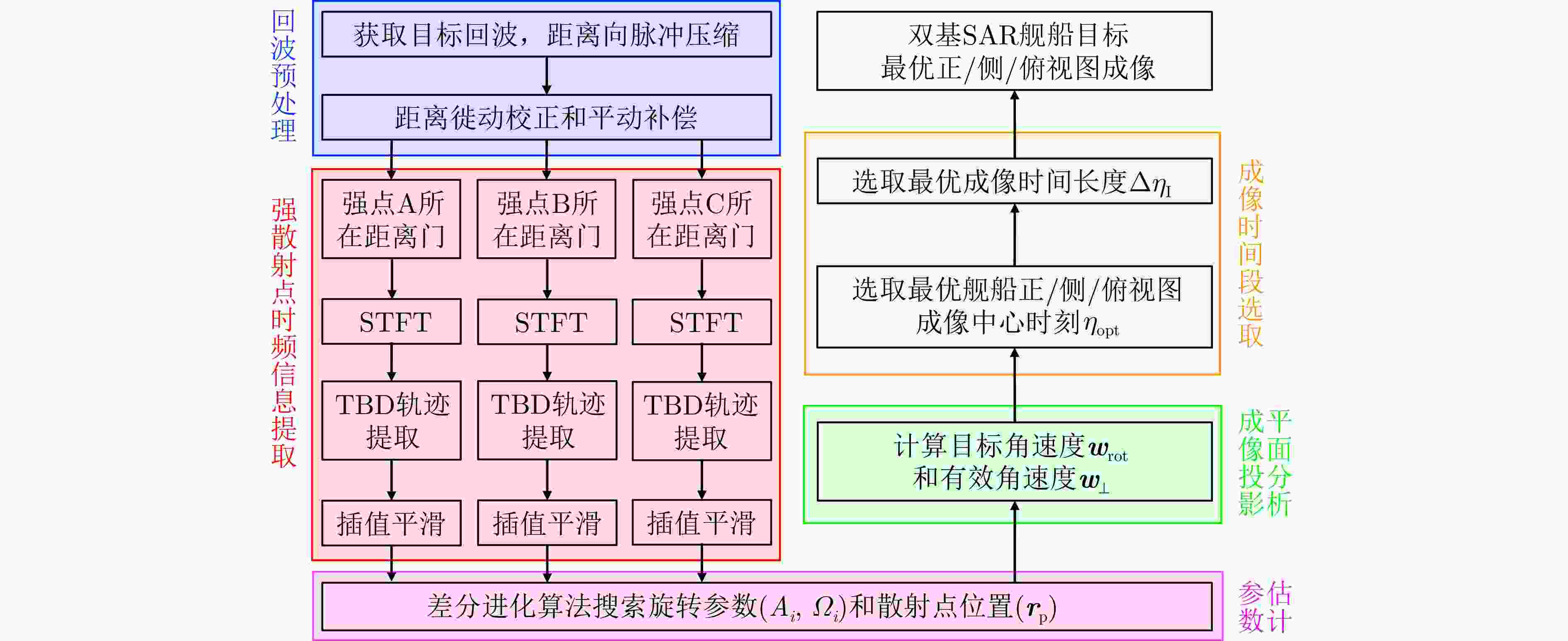
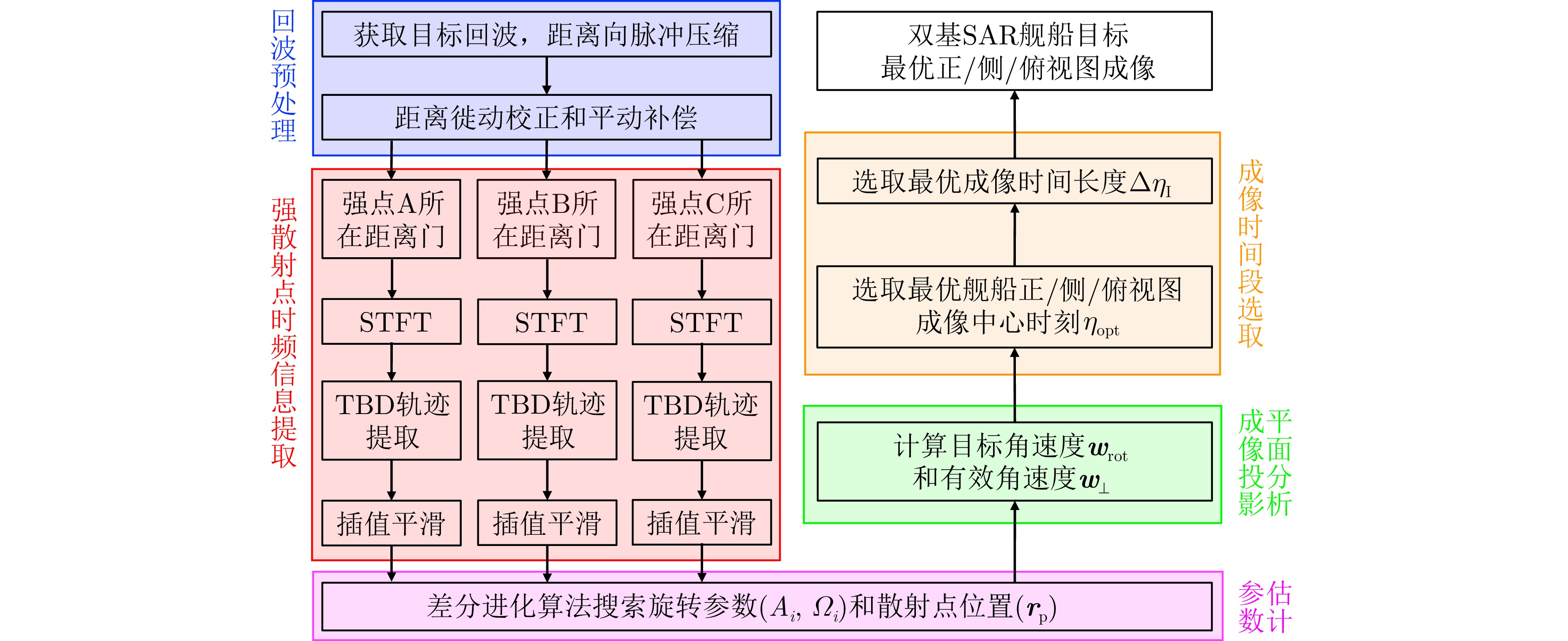
图 3 双基SAR舰船目标成像时段最优成像处理
Figure 3. Flow chat of imaging time optimication method for shop target for bistatic SAR
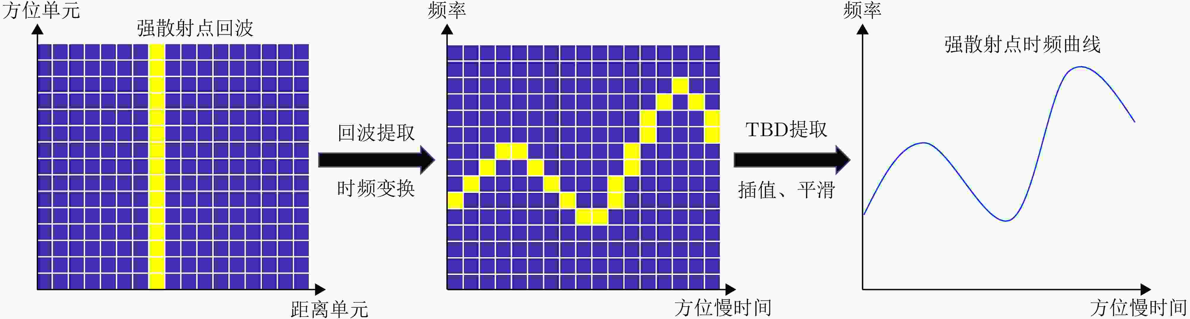
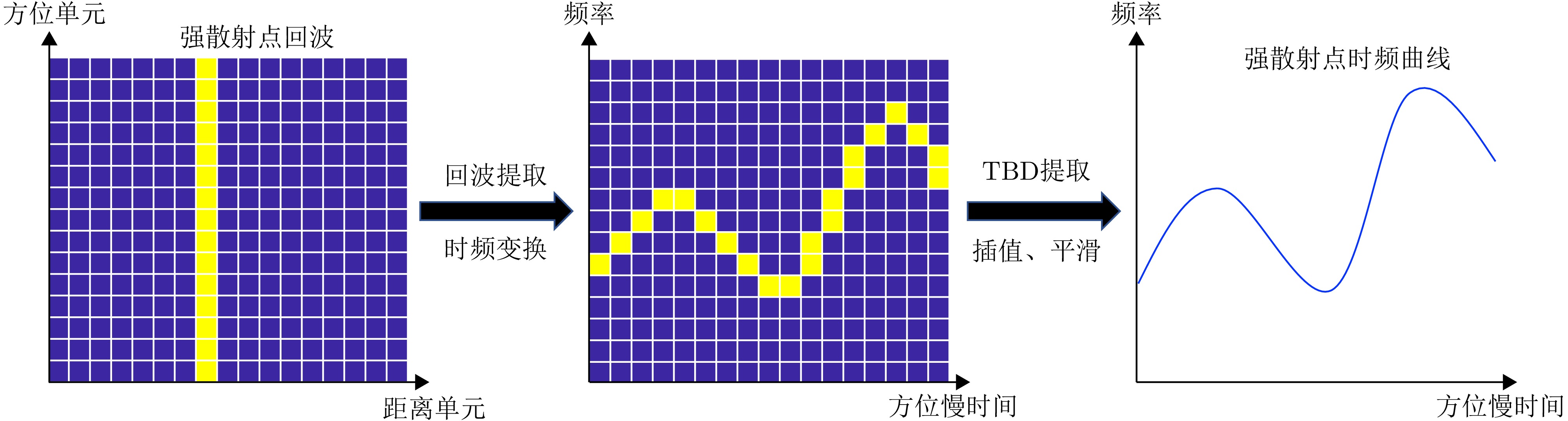
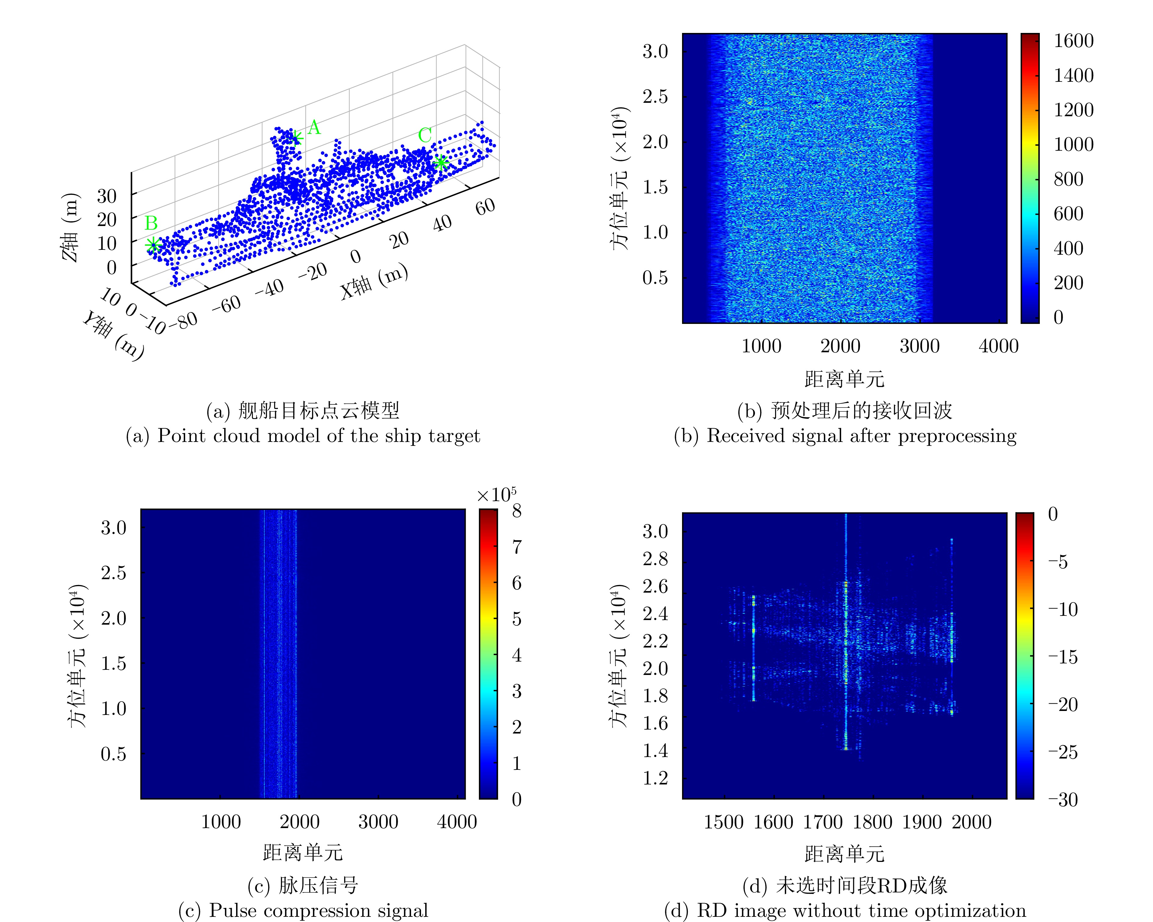
图 4 强散射点时频信息提取示意图
Figure 4. Schematic of time-frequency data extraction of strong scatterers
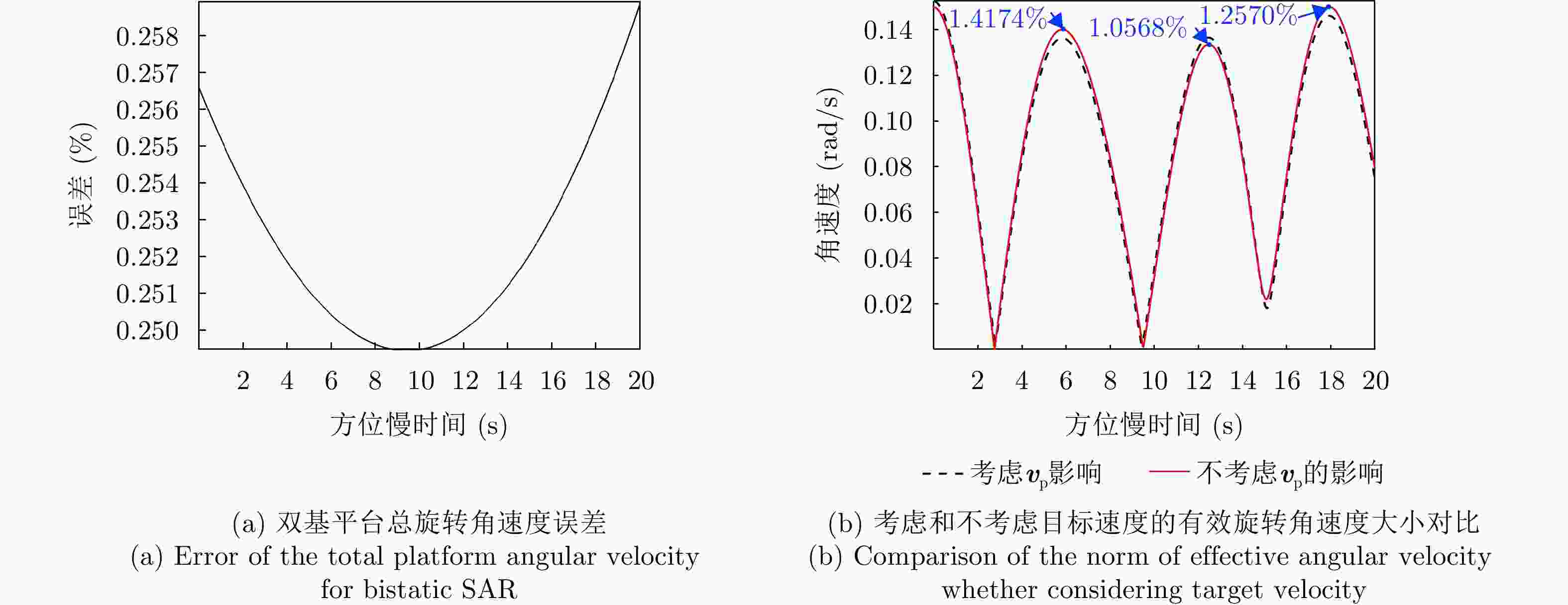
图 8 实际参数与本方法公式推导的差异
Figure 8. Comparison between actual parameters and the ones deduced by this method
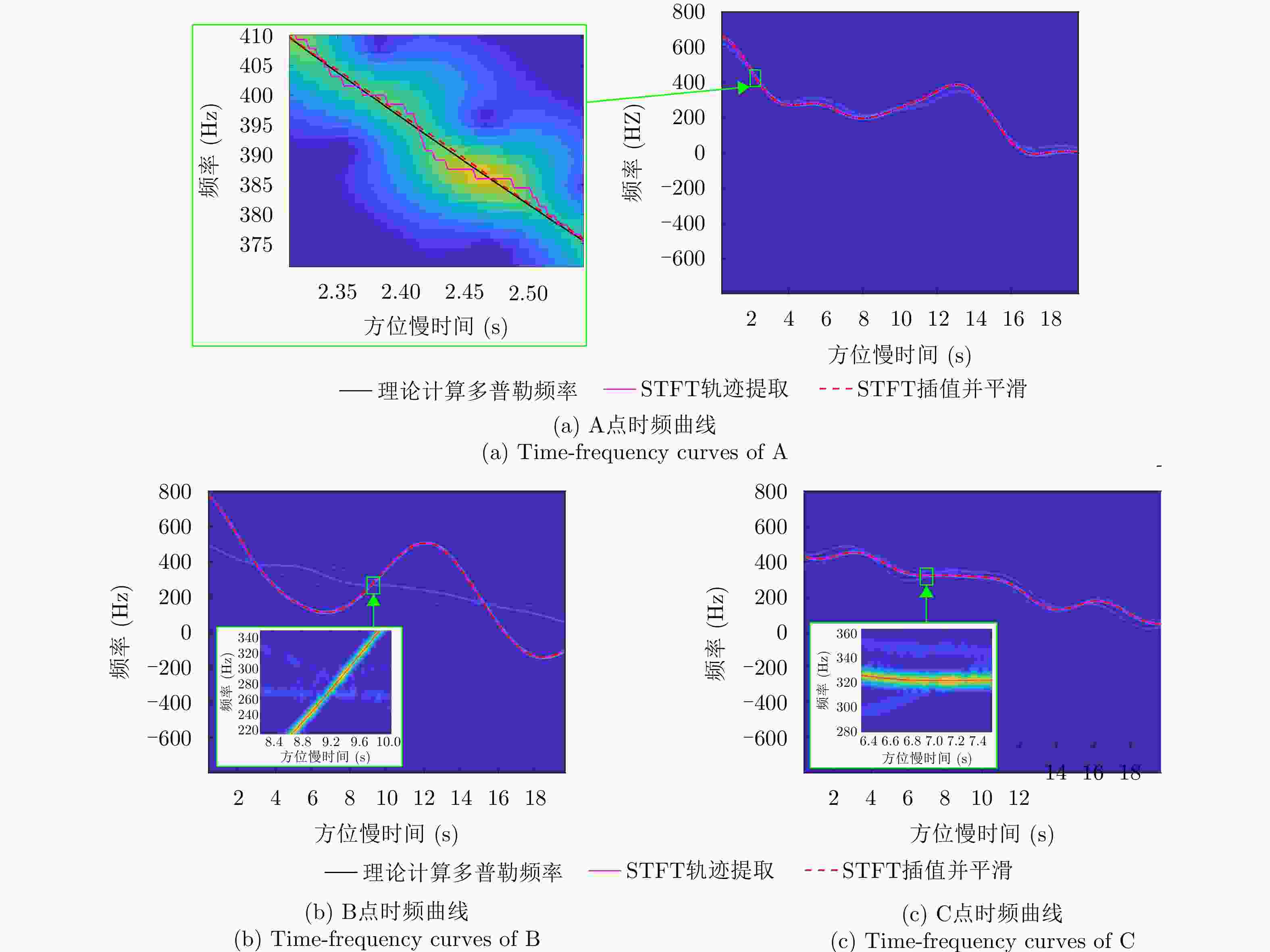
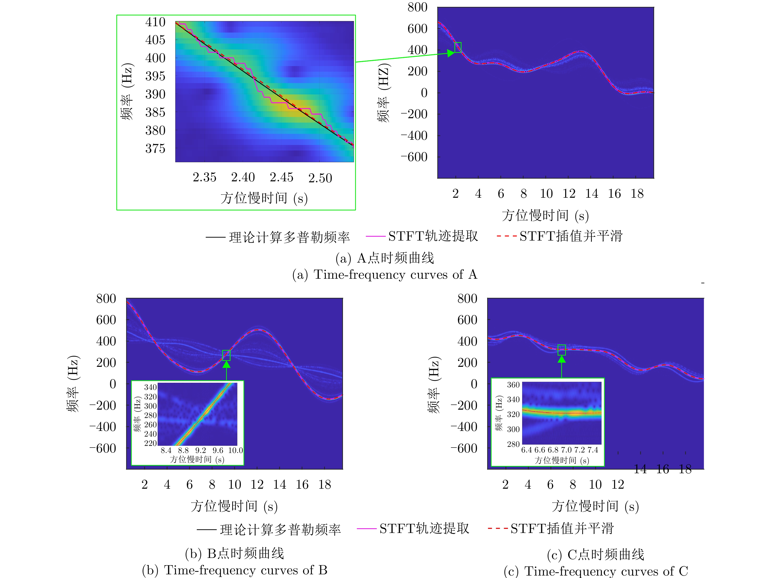
图 9 强散射点STFT结果,STFT峰值轨迹提取、插值并平滑曲线以及理论时频曲线
Figure 9. STFT results of strong scatterers, curves of trace extraction from STFT results after interpolation and smoothing, as well as theoretical time-frequency curves
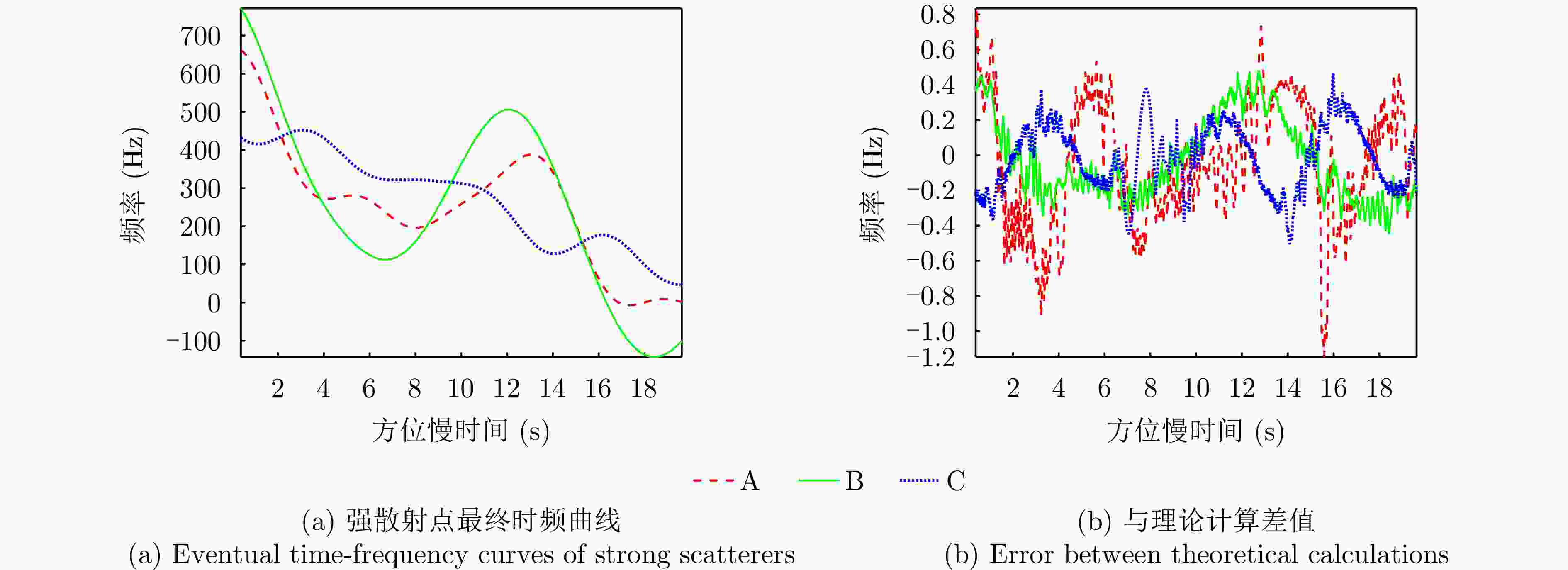
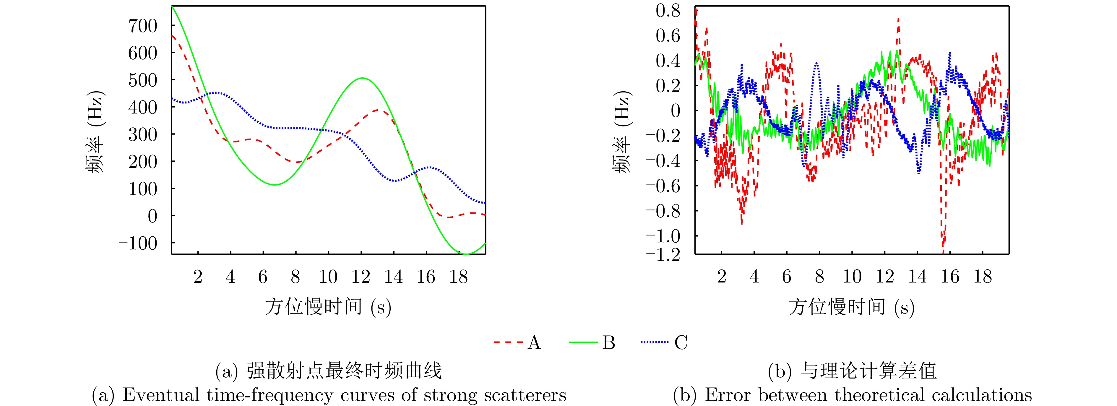
图 10 $ \mathrm{A} $, $ \mathrm{B} $, $ \mathrm{C} $点时频分析结果与误差
Figure 10. Results and errors of time-frequency curves of $ \mathrm{A} $, $ \mathrm{B} $ and $ \mathrm{C} $

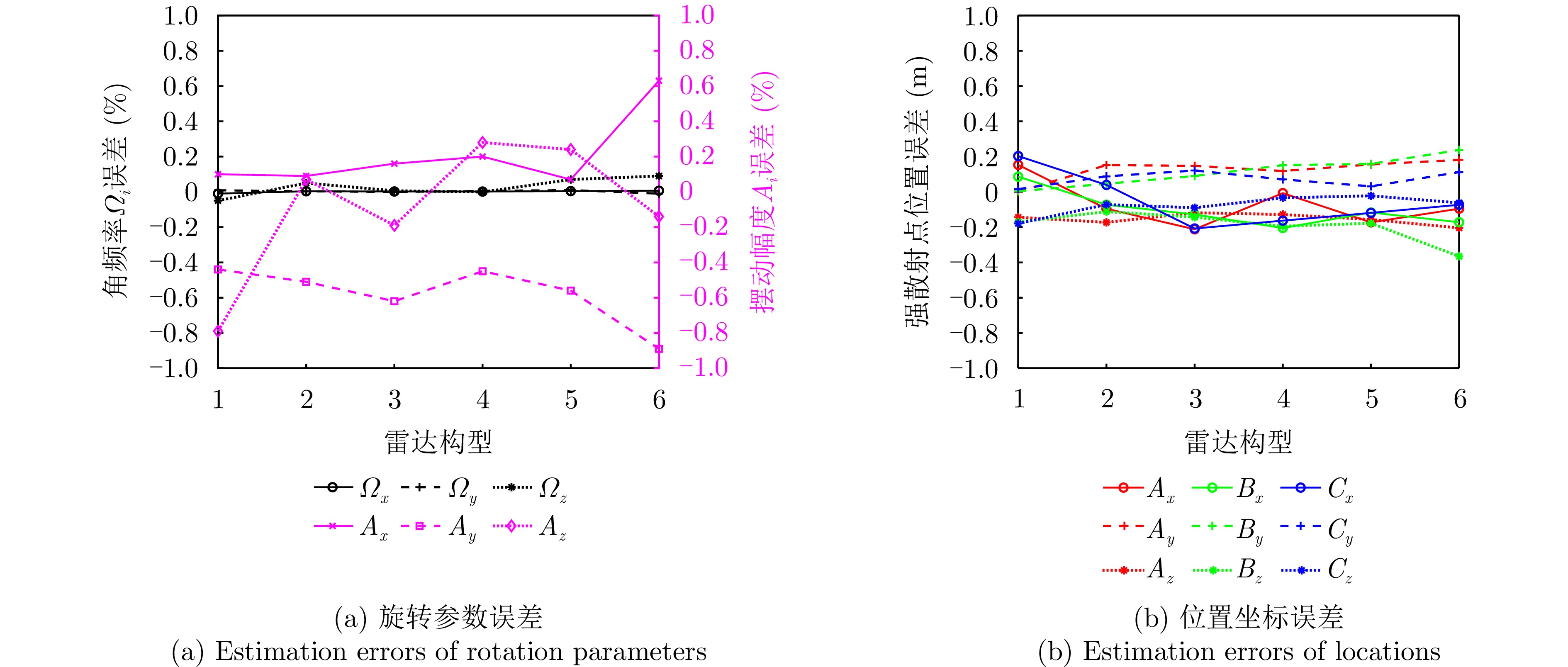
图 12 不同双基构型下强散射点参数估计误差
Figure 12. Estimation errors of strong scatterers of different bistatic SAR configurations
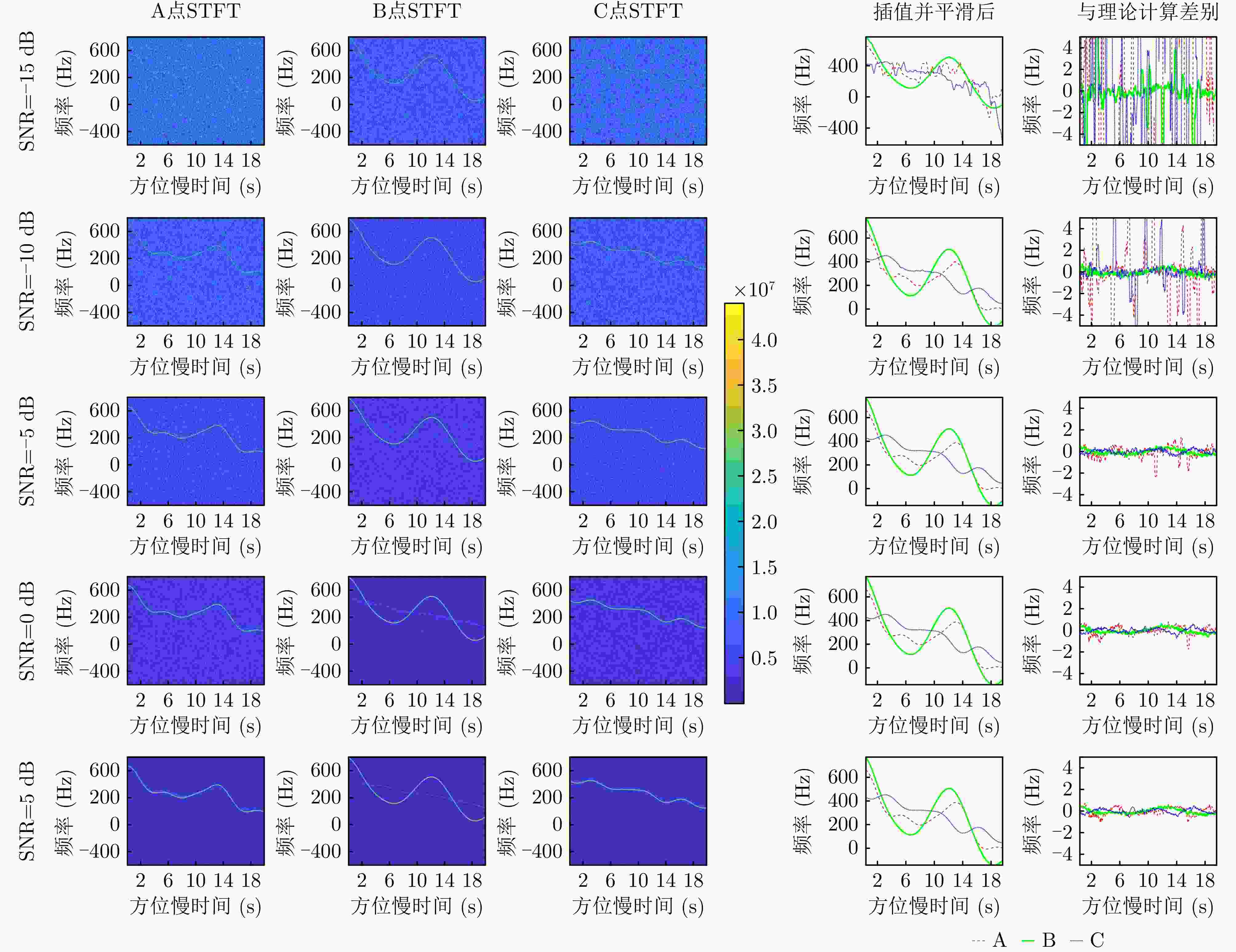
图 13 在不同噪声环境下的3个强散射点时频曲线
Figure 13. Time-frequency curves of three strong scatterers under conditions of noise with different $ \mathrm{S}\mathrm{N}\mathrm{R} $
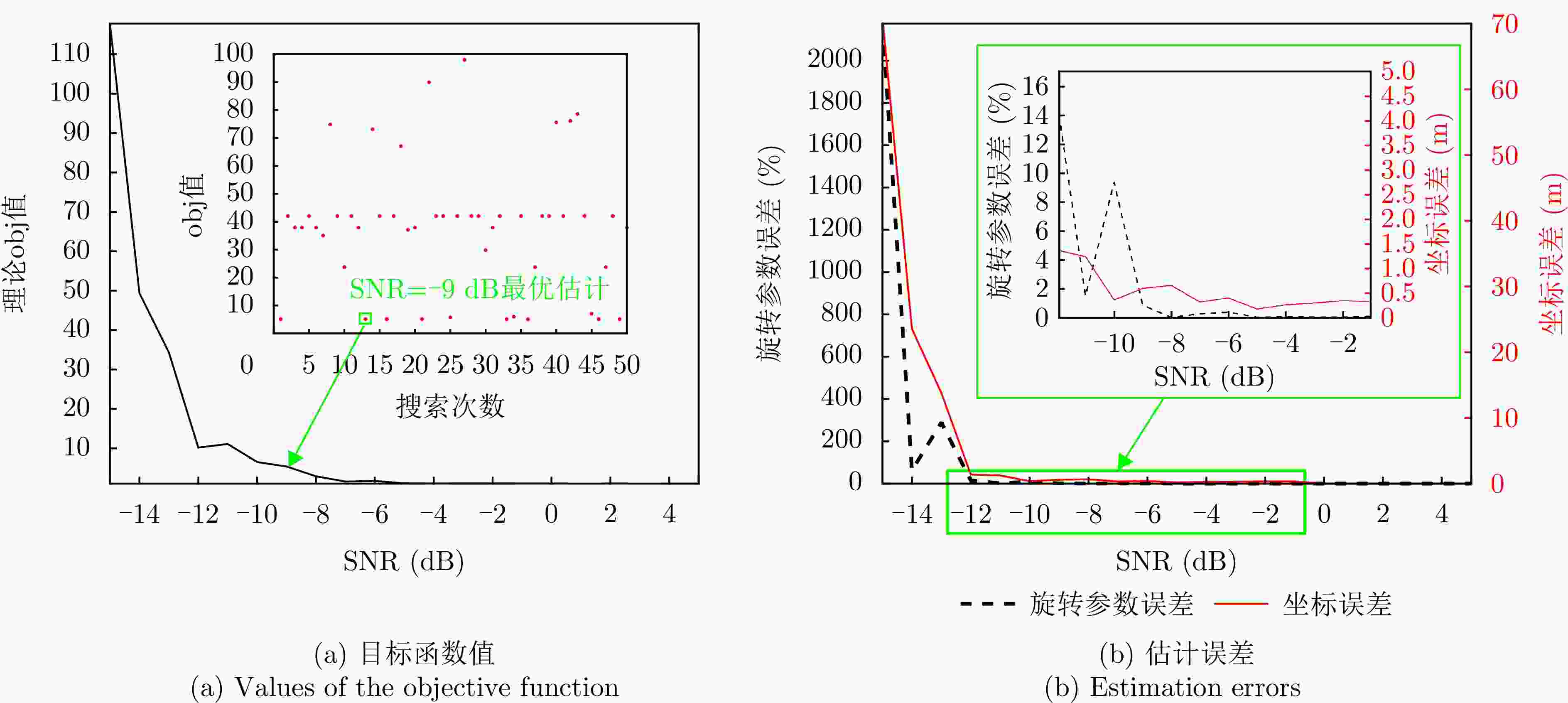
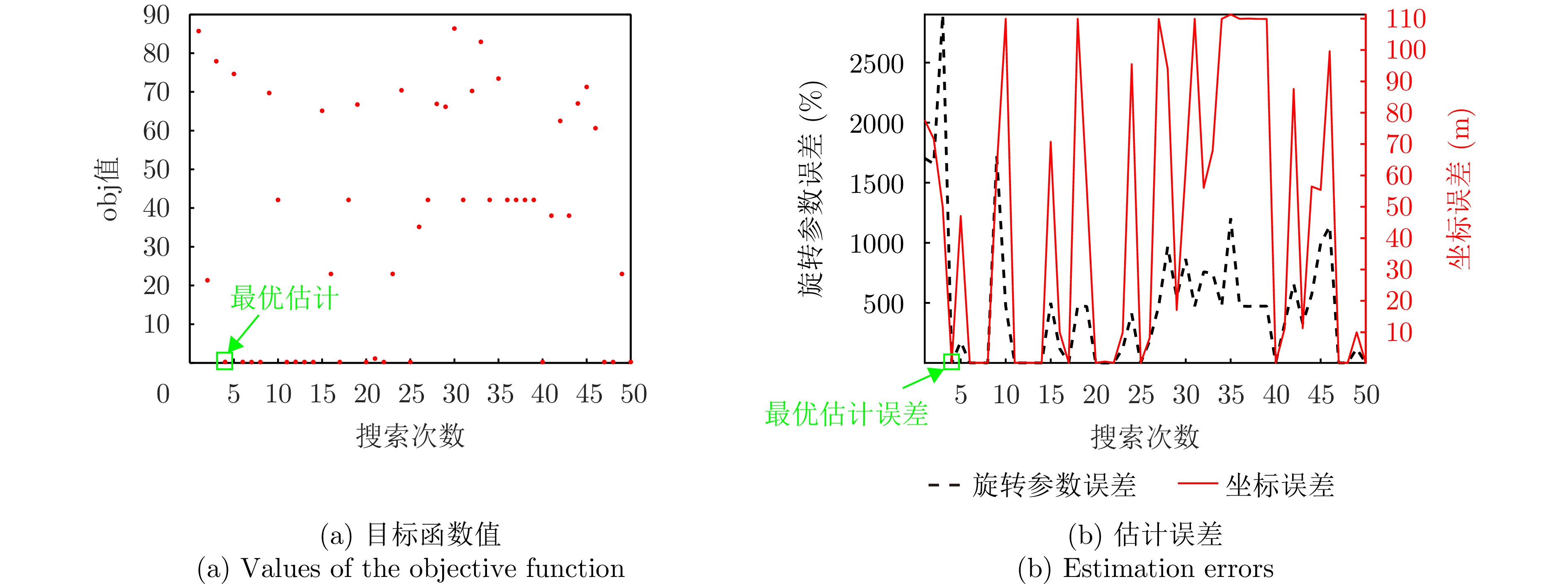
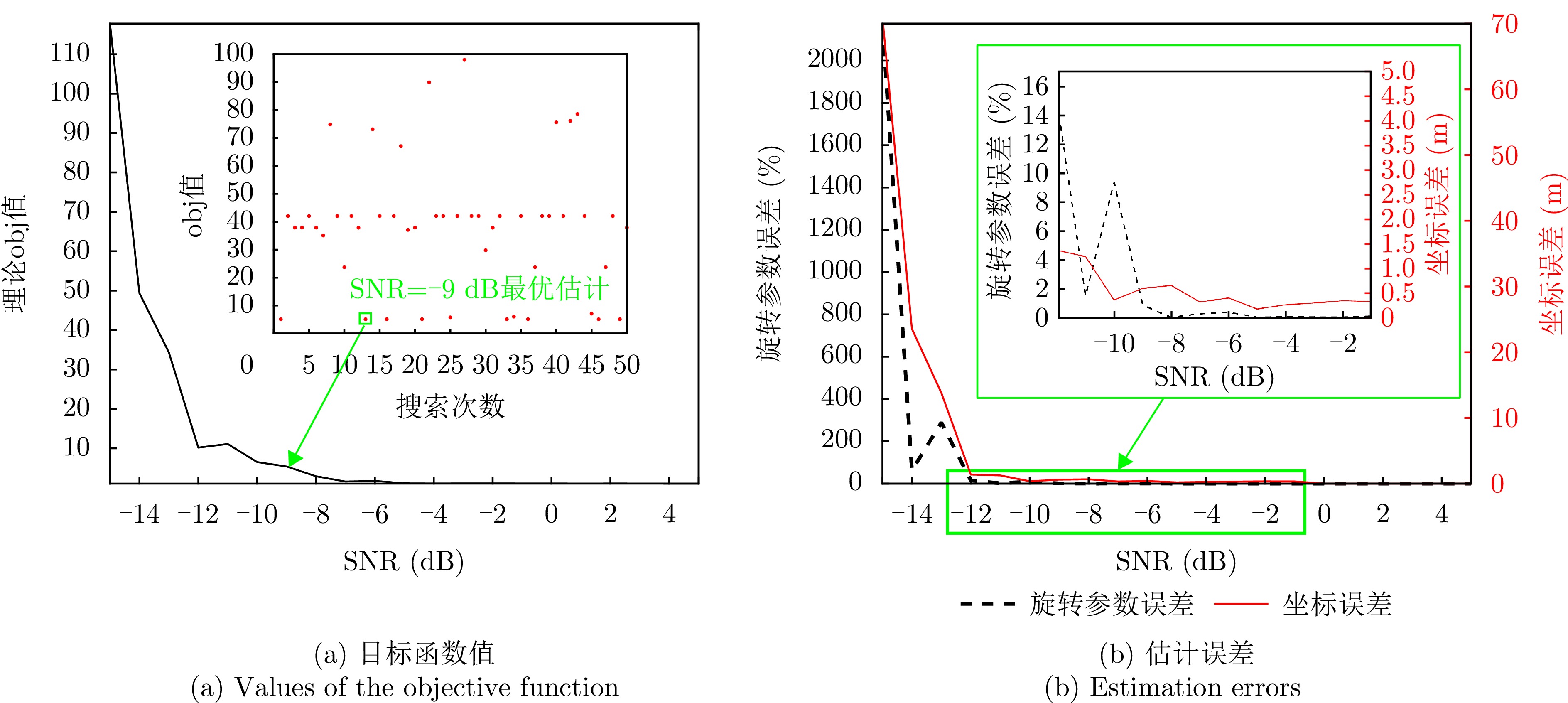
图 14 不同噪声环境下DE估计结果
Figure 14. Estimation results by DE algorithm under conditions of noise with different $ \mathrm{S}\mathrm{N}\mathrm{R} $
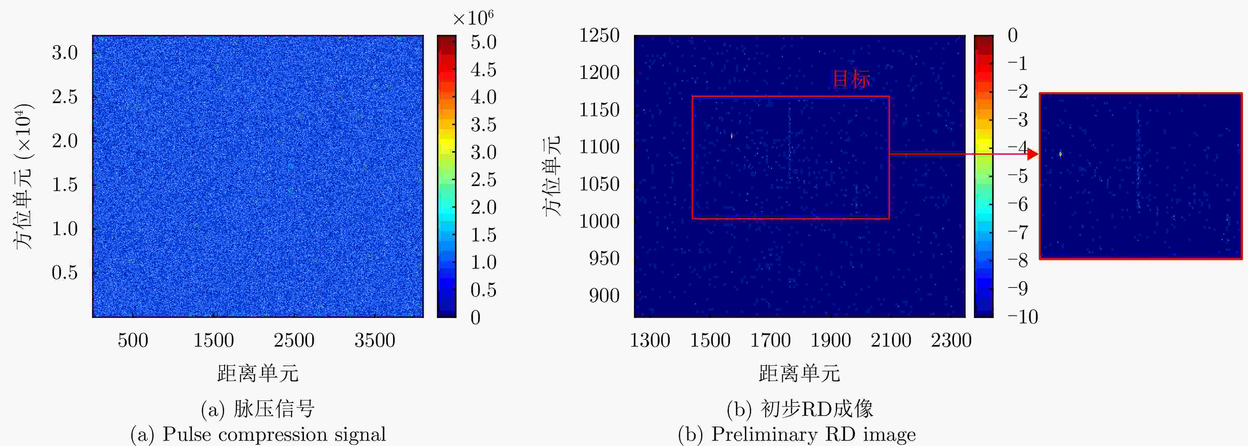
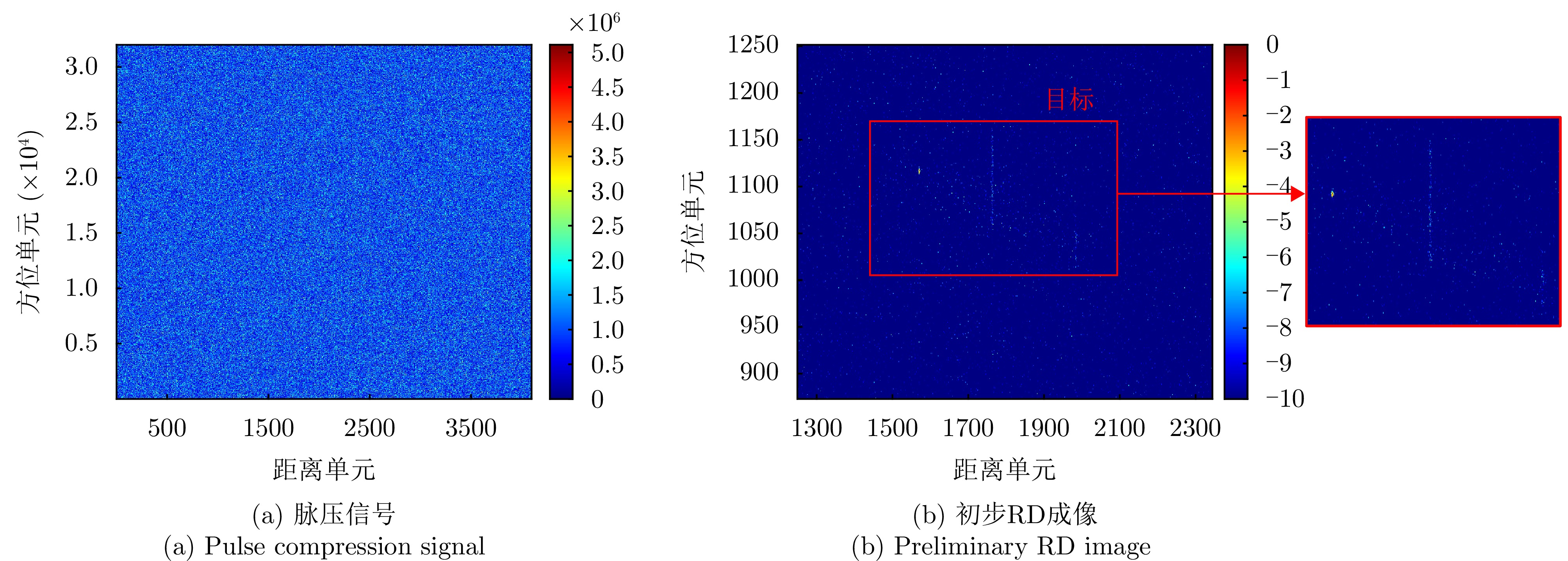
图 15 $ \mathrm{S}\mathrm{N}\mathrm{R}=-9 $ dB条件下的信号
Figure 15. Signals when $ \mathrm{S}\mathrm{N}\mathrm{R}=-9 $ dB
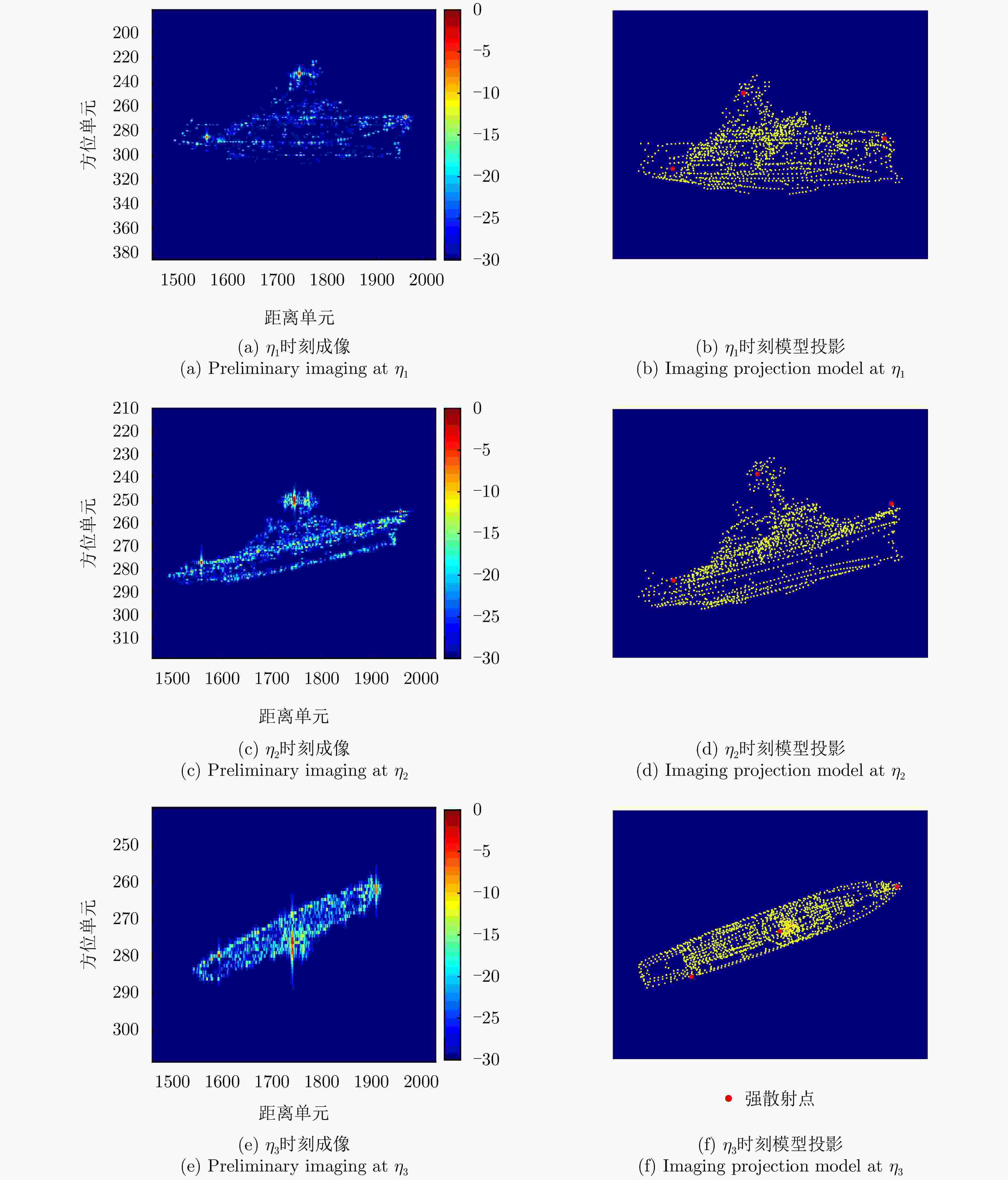
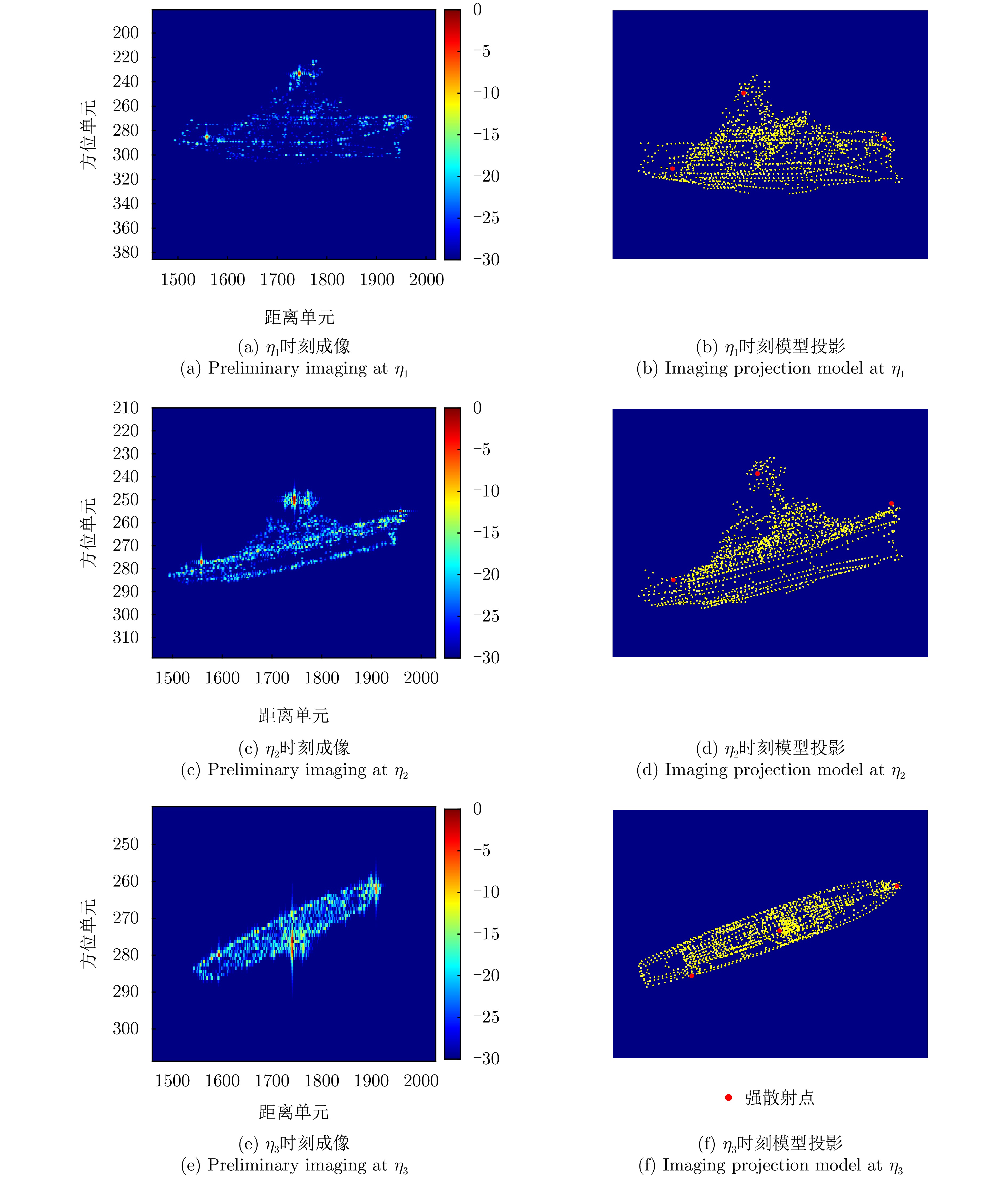
图 17 不同时刻目标初步RD成像与其对应IPP上点云模型投影
Figure 17. Preliminary imaging results at different time centers and imaging projection models on the corresponding IPPs
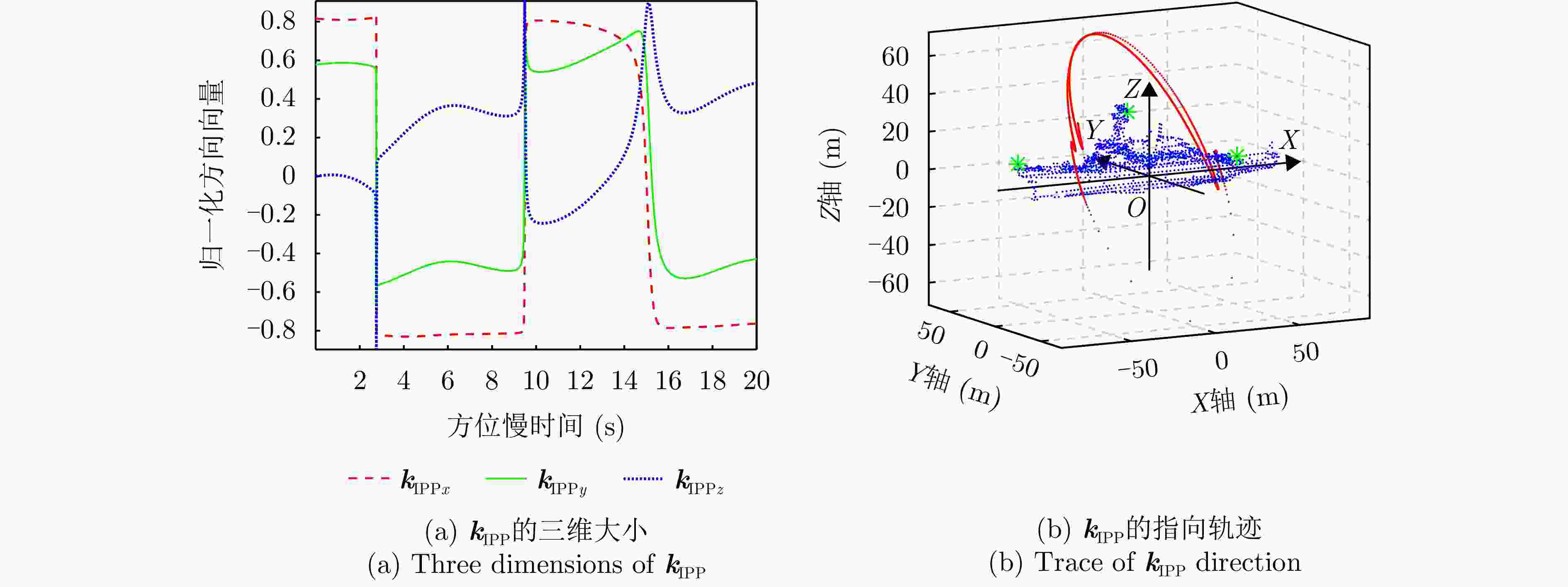
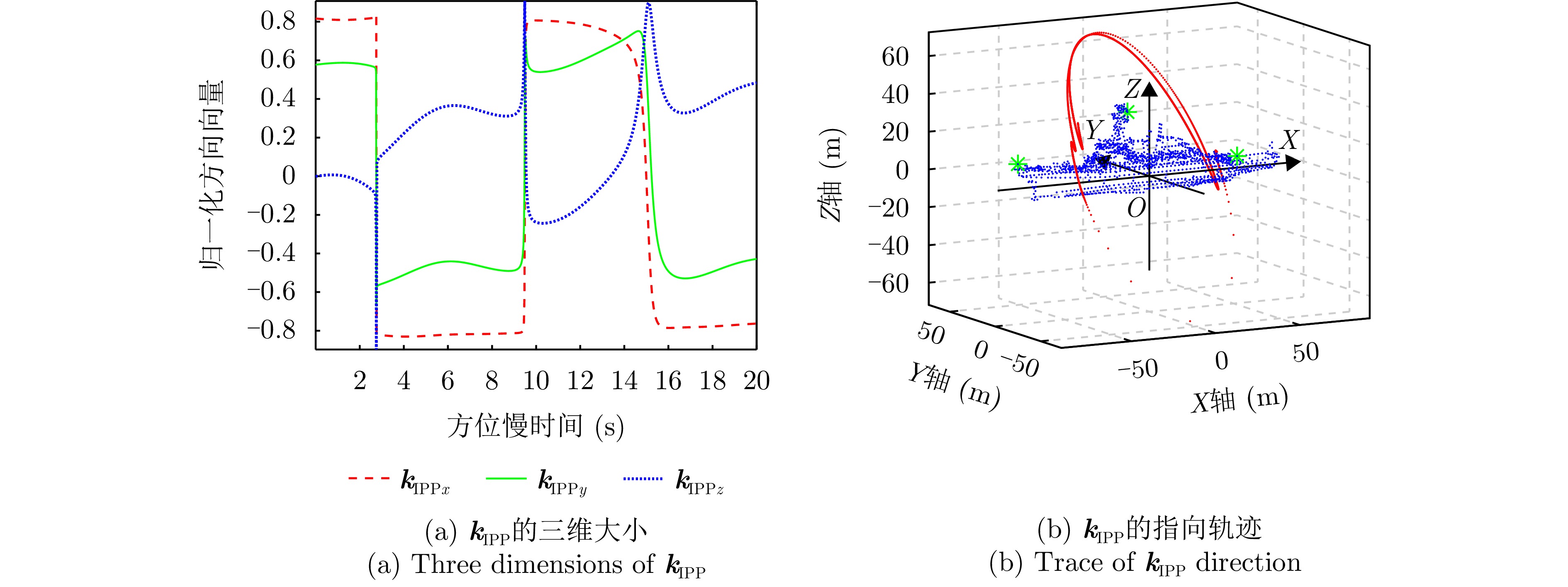
图 18 估计IPP法向量$ {\boldsymbol{k}}_{\mathrm{I}\mathrm{P}\mathrm{P}}\left(\eta \right) $
Figure 18. Estimated normal vector of IPP $ {\boldsymbol{k}}_{\mathrm{I}\mathrm{P}\mathrm{P}}\left(\eta \right) $
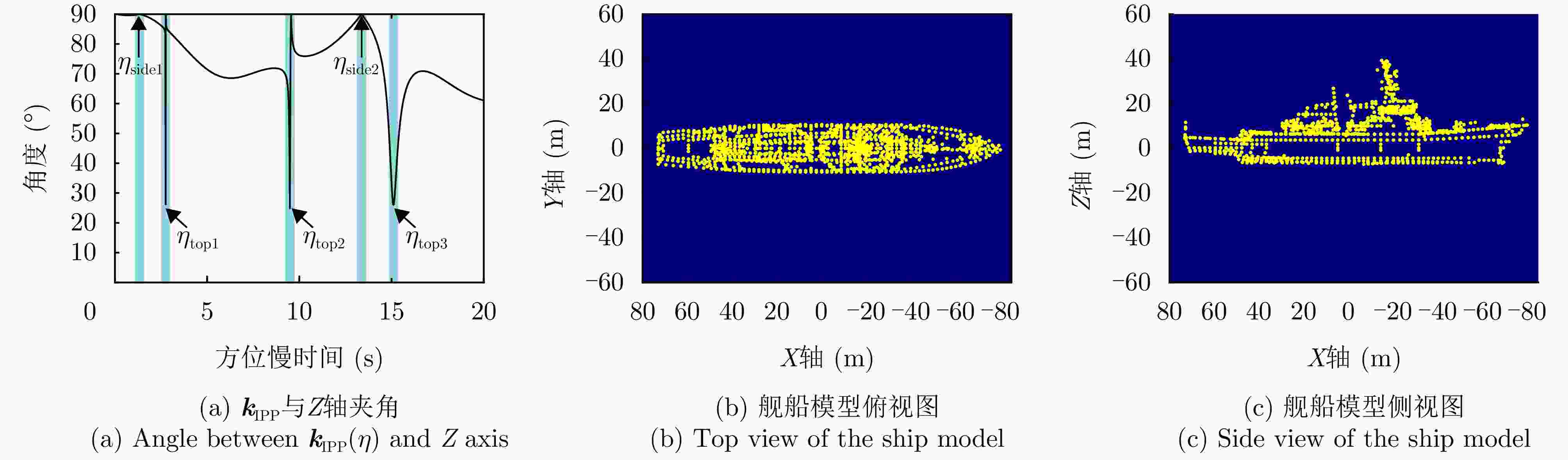
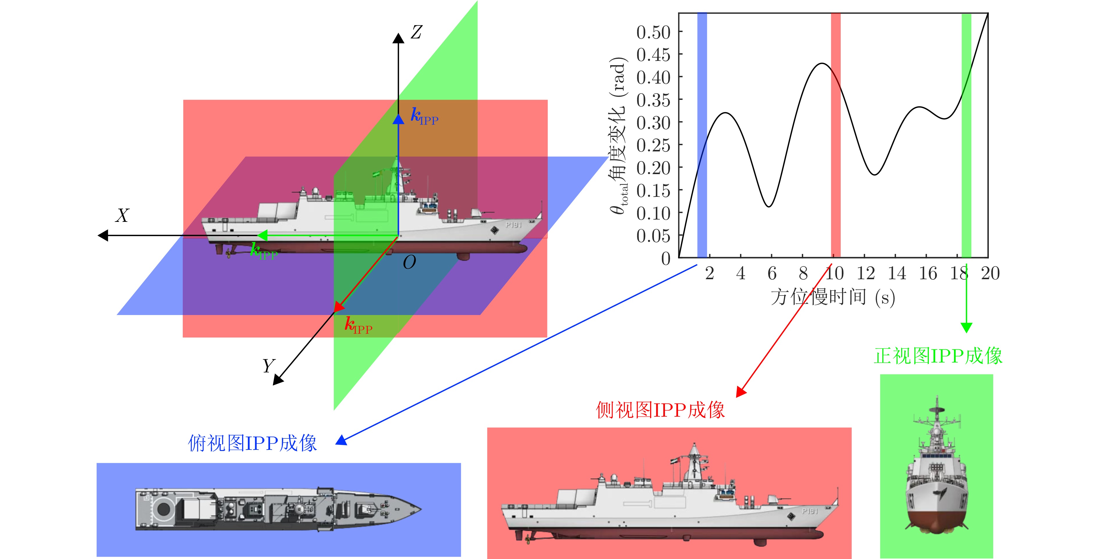
图 19 成像中心时刻与预期目标视图
Figure 19. Imaging time centers and desired results of different imaging views
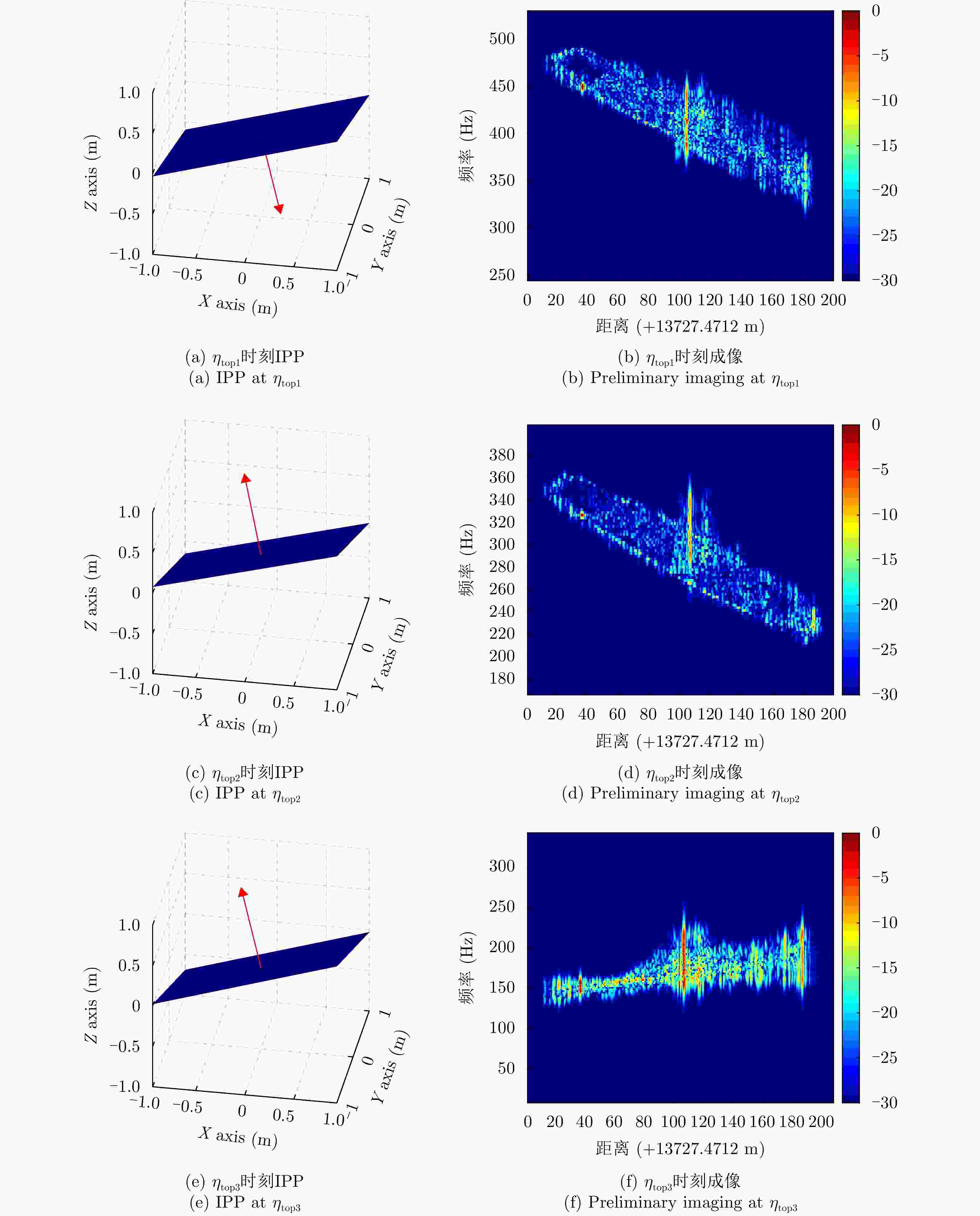
图 20 俯视图成像时刻IPP与初步RD成像结果
Figure 20. IPP and preliminary RD imaging results for top view
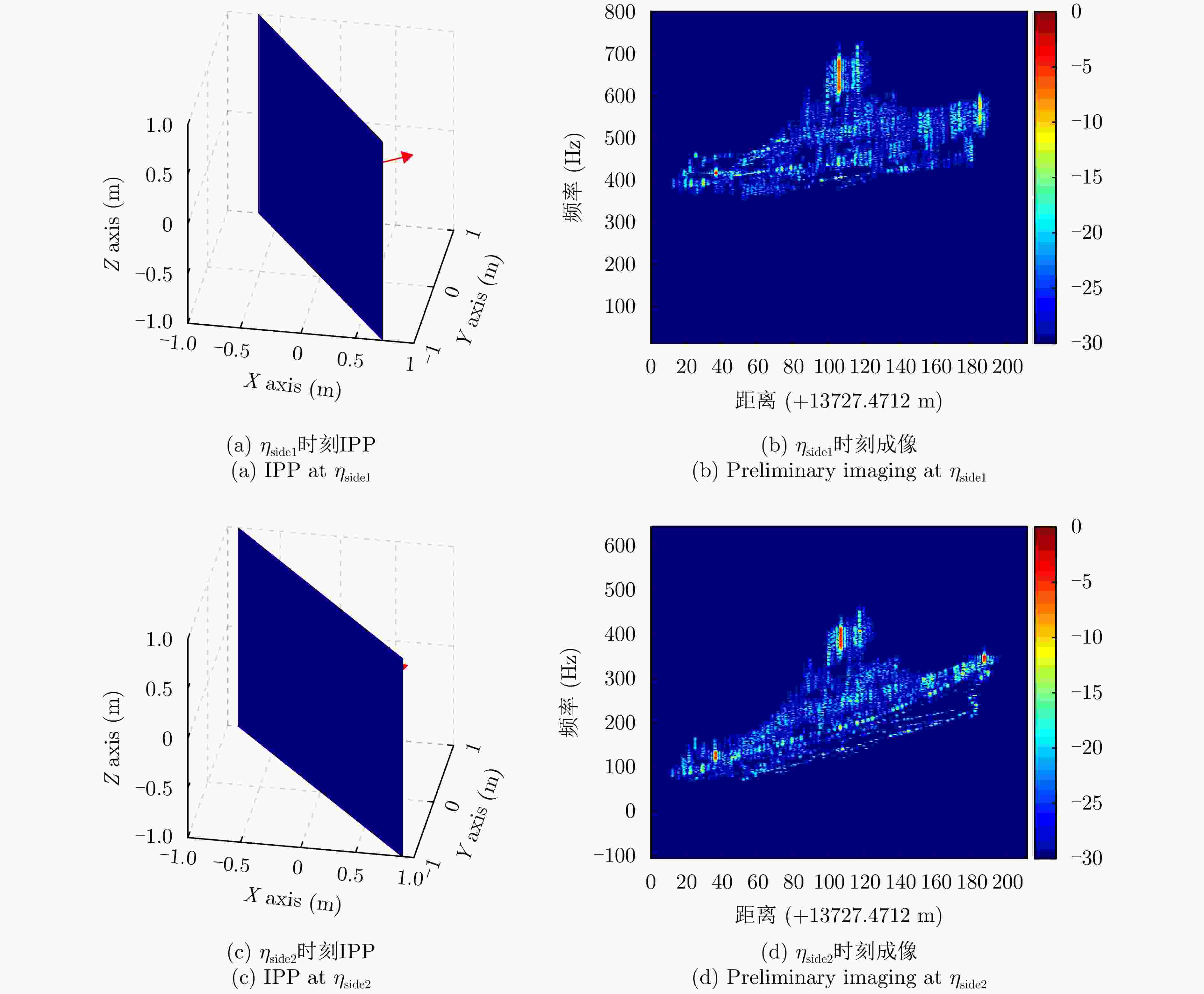
图 21 侧视图成像时刻IPP与初步RD成像结果
Figure 21. IPP and preliminary RD imaging results for side view
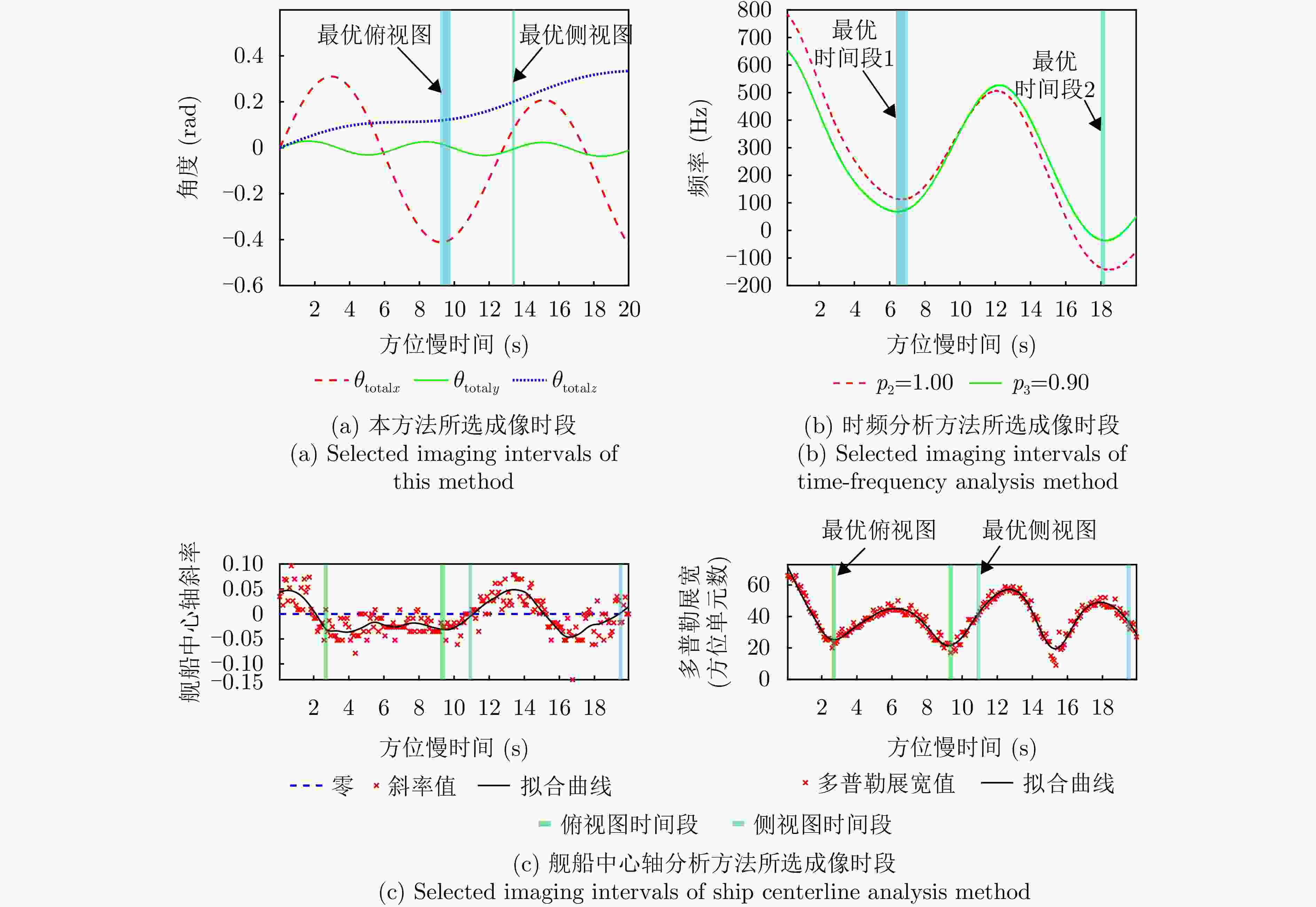
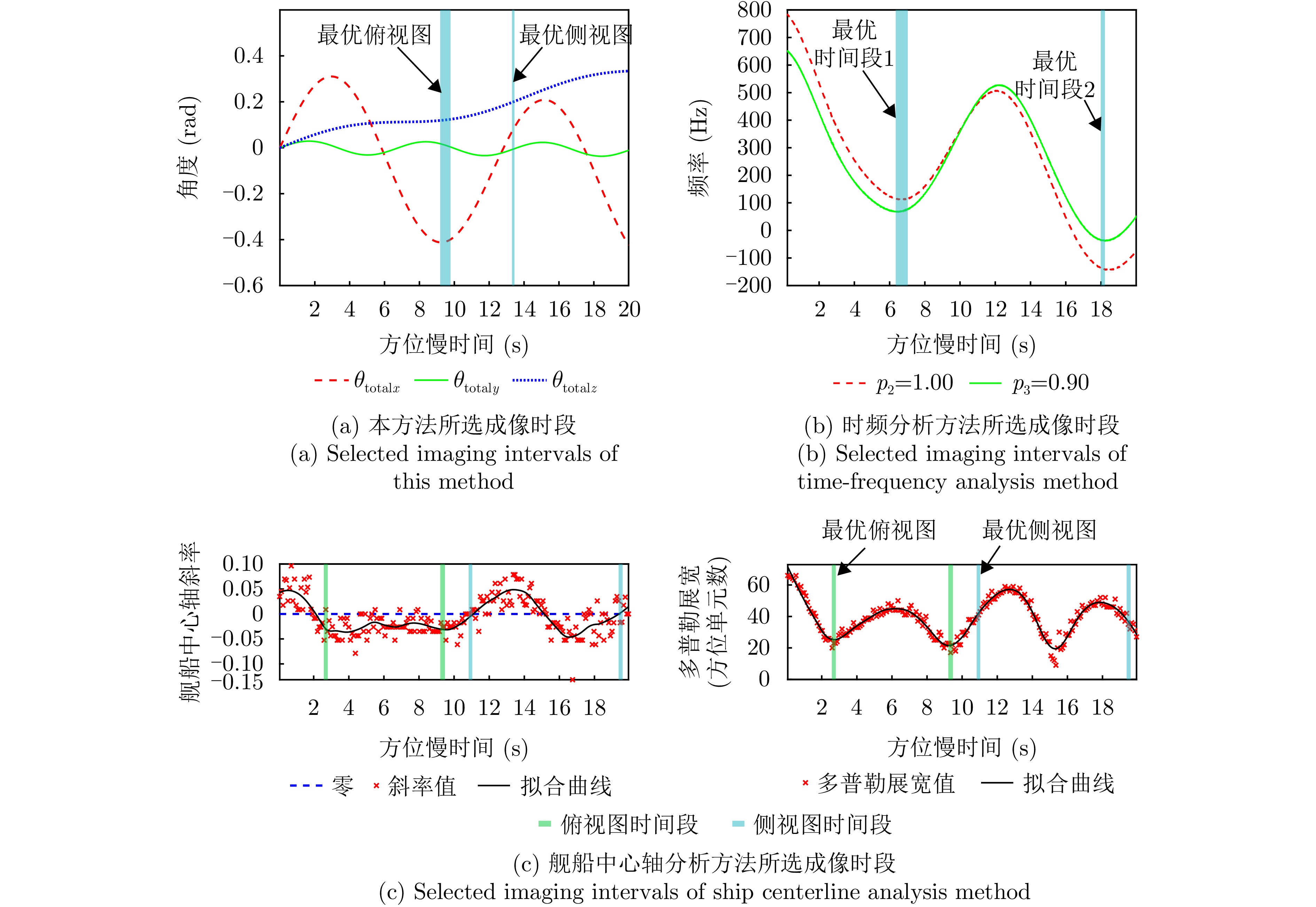
图 22 本方法与其他方法所选最优成像时段
Figure 22. Selected optimal time intervals of the proposed method and other methods
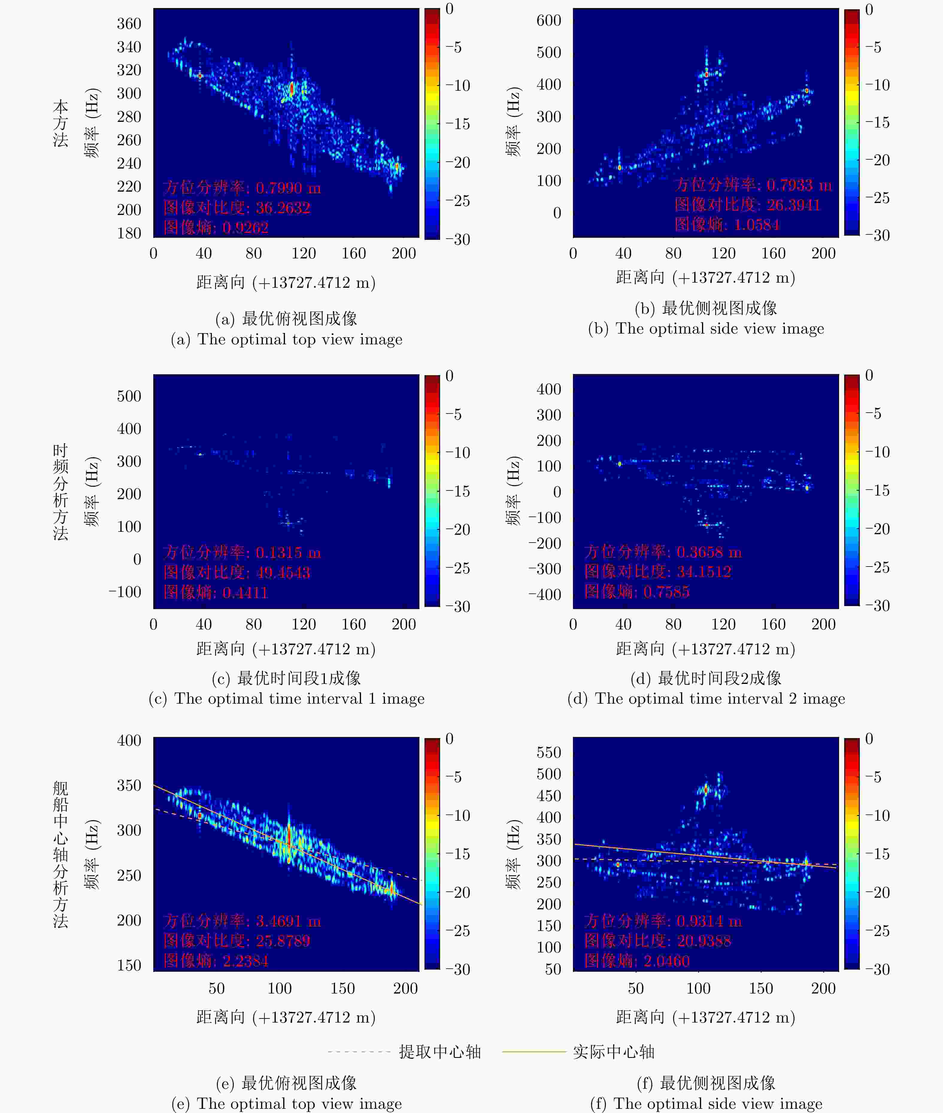
图 23 本方法与其他方法成像处理结果
Figure 23. Imaging results of the proposed methods and other methods
表 1 雷达参数与舰船运动参数
Table 1. Parameters of bistatic SAR and the ship target
参数 符号 数值 载波频率 $ {f}_{\mathrm{c}} $ 9.6 GHz 带宽 B 200 MHz 脉冲重复频率 $ \mathrm{P}\mathrm{R}\mathrm{F} $ 1600 Hz 采样频率 $ {f}_{\mathrm{s}} $ 800 MHz 总观测时间 $ {T}_{\mathrm{t}\mathrm{o}\mathrm{t}\mathrm{a}\mathrm{l}} $ 20 s 发射平台位置 $ {\boldsymbol{r}}_{\mathrm{T}} $ [4000, –2600, 2000]T m 发射平台速度 $ {\boldsymbol{v}}_{\mathrm{T}} $ [10, 57, 20]T m·s–1 接收平台位置 $ {\boldsymbol{r}}_{\mathrm{R}} $ [2000, –8000, 3000]T m 接收平台速度 $ {\boldsymbol{v}}_{\mathrm{R}} $ [57, 15, 15]T m·s–1 目标速度 $ {\boldsymbol{v}}_{\mathrm{p}} $ [20, 10, 0]T m·s–1 目标散射点位置 $ {\boldsymbol{r}}_{\mathrm{A}} $ [–78.0, 0.0, 13.0]T m $ {\boldsymbol{r}}_{\mathrm{B}} $ [–13.0, 0.0, 35.0]T m $ {\boldsymbol{r}}_{\mathrm{C}} $ [–47.0, –9.3, 8.0]T m  下载: 导出CSV
表 2 舰船旋转参数
Table 2. Rotation parameters of the ship target
维度 摆动幅度$ {{A}}_{{i}} $ (rad) 角频率$ {{\varOmega }}_{{i}} $ (rad·s–1) U轴(横滚) 0.3351 0.5150 V轴(俯仰) 0.0297 0.9378 W轴(偏航) 0.0332 0.4425
下载: 导出CSV
表 3 舰船旋转参数估计结果与误差
Table 3. Estimation results and errors of rotation parameters of the ship target
维度 摆动幅度$ {{A}}_{{i}} $(rad) 误差(%) 角频率$ {{\varOmega }}_{{i}} $(rad·s–1) 误差(%) U轴(横滚) $ 0.3354 $ $ +0.08 $ $ 0.5150 $ $ +0.00 $ V轴(俯仰) $ 0.0294 $ $ -0.88 $ $ 0.9378 $ $ +0.00 $ W轴(偏航) $ 0.0331 $ $ -0.16 $ $ 0.4426 $ $ +0.03 $
下载: 导出CSV
表 4 强散射点位置参数估计结果与误差
Table 4. Estimation results and errors of locations of strong scatterers
散射点 坐标(m) 误差(m) $ \mathrm{A} $ $ {\left[-78.2718, 0.2639, 12.8119\right]}^{\rm{T}} $ $ {\left[-0.2718, 0.2639, -0.1881\right]}^{\rm{T}} $ $ \mathrm{B} $ $ {\left[-13.2415,\mathrm{ }0.1169,\mathrm{ }34.8537\right]}^{\rm{T}} $ $ {\left[-0.2415,\mathrm{ }0.1169,-0.1463\right]}^{\rm{T}} $ $ \mathrm{C} $ $ {\left[46.9313, -9.2144, 7.9404\right]}^{\rm{T}} $ $ {\left[-0.0687, 0.0856, -0.0596\right]}^{\rm{T}} $
下载: 导出CSV
表 5 不同双基SAR构型的参数
Table 5. Radar parameters of different bistatic SAR configurations
雷达构型 $ {\boldsymbol{r}}_{\mathrm{T}} $(m) $ {\boldsymbol{r}}_{\mathrm{R}} $(m) $ {\boldsymbol{v}}_{\mathrm{T}} $(m·s–1) $ {\boldsymbol{v}}_{\mathrm{R}} $(m·s–1) 1 $ {\left[-1000,-2600,\mathrm{ }3000\right]}^{\rm{T}} $ $ {\left[-2000,\mathrm{ }2000,\mathrm{ }3000\right]}^{\rm{T}} $ $ {\left[10, 57, 20\right]}^{\rm{T}} $ $ {\left[57, 15, 15\right]}^{\rm{T}} $ 2 $ {\left[4000,-2600,\mathrm{ }4000\right]}^{\rm{T}} $ $ {\left[0,\mathrm{ }- 8000,\mathrm{ }3000\right]}^{\rm{T}} $ $ {\left[10, 57, 20\right]}^{\rm{T}} $ $ {\left[57, 15, 15\right]}^{\rm{T}} $ 3 $ {\left[4000, -2600, 2000\right]}^{\rm{T}} $ $ {\left[2000, -8000, 3000\right]}^{\rm{T}} $ $ {\left[30, 30, 10\right]}^{\rm{T}} $ $ {\left[40, 40, 0\right]}^{\rm{T}} $ 4 $ {\left[4000, -2600, 2000\right]}^{\rm{T}} $ $ {\left[2000, -8000, 3000\right]}^{\rm{T}} $ $ {\left[30, -10, 0\right]}^{\rm{T}} $ $ {\left[30, -20, 0\right]}^{\rm{T}} $ 5 $ {\left[3000,-\mathrm{2600,3000}\right]}^{\rm{T}} $ $ {\left[4000,-\mathrm{8000,3000}\right]}^{\rm{T}} $ $ {\left[-10,\mathrm{ }50,\mathrm{ }0\right]}^{\rm{T}} $ $ {\left[50,-20,0\right]}^{\rm{T}} $ 6 $ {\left[4000,-\mathrm{2600,2000}\right]}^{\rm{T}} $ $ {\left[-4000,-\mathrm{8000,2000}\right]}^{\rm{T}} $ $ {\left[25,-58,\mathrm{ }0\right]}^{\rm{T}} $ $ {\left[-33,-25,\mathrm{ }2\right]}^{\rm{T}} $
下载: 导出CSV
表 6 各中心时刻成像指标
Table 6. Image indices of imaging results at different time centers
中心时刻 方位分辨率(m) 图像对比度 图像锐度 图像熵 归一化互信息(NMI) $ {\eta }_{1} $ $ 0.3456 $ $ 73.4218 $ $ 1.1672\times {10}^{11} $ $ 2.0656 $ $ 0.3561 $ $ {\eta }_{2} $ $ 0.6558 $ $ 62.8259 $ $ 1.0108\times {10}^{11} $ $ 2.4770 $ $ 0.4961 $ $ {\eta }_{3} $ $ 1.8712 $ $ 63.7224 $ $ 7.7467\times {10}^{10} $ $ 2.3724 $ $ 0.6292 $
下载: 导出CSV
表 7 俯视图各中心时刻成像指标
Table 7. Image indices of imaging results at different time centers for top view
中心时刻 归一化互信息(NMI) 图像对比度 图像熵 $ {\eta }_{\mathrm{t}\mathrm{o}\mathrm{p}1} $ 0.3778 18.5044 3.0481 $ {\eta }_{\mathrm{t}\mathrm{o}\mathrm{p}2} $ 0.3161 24.4196 2.3900 $ {\eta }_{\mathrm{t}\mathrm{o}\mathrm{p}3} $ 0.1492 14.3753 2.6636
下载: 导出CSV
表 8 侧视图中心时刻成像指标
Table 8. Image indices of imaging results at different time centers for side view
中心时刻 归一化互信息(NMI) 图像对比度 图像熵 $ {\eta }_{\mathrm{s}\mathrm{i}\mathrm{d}\mathrm{e}1} $ 0.4119 14.8815 2.0307 $ {\eta }_{\mathrm{s}\mathrm{i}\mathrm{d}\mathrm{e}2} $ 0.4812 16.2234 1.9778
下载: 导出CSV
-
[1] BROWN W M and PORCELLO L J. An introduction to synthetic-aperture radar[J]. IEEE Spectrum, 1969, 6(9): 52–62. doi: 10.1109/MSPEC.1969.5213674. [2] LI Zhongyu, HUANG Chuan, SUN Zhichao, et al. BeiDou-based passive multistatic radar maritime moving target detection technique via space-time hybrid integration processing[J]. IEEE Transactions on Geoscience and Remote Sensing, 2022, 60: 5802313. doi: 10.1109/TGRS.2021.3128650. [3] YANG Qing, LI Zhongyu, LI Junao, et al. A novel bistatic SAR maritime ship target imaging algorithm based on cubic phase time-scaled transformation[J]. Remote Sensing, 2023, 15(5): 1330. doi: 10.3390/rs15051330. [4] 武俊杰, 孙稚超, 吕争, 等. 星源照射双/多基地SAR成像[J]. 雷达学报, 2023, 12(1): 13–35. doi: 10.12000/JR22213.WU Junjie, SUN Zhichao, LV Zheng, et al. Bi/multi-static synthetic aperture radar using spaceborne illuminator[J]. Journal of Radars, 2023, 12(1): 13–35. doi: 10.12000/JR22213. [5] WU Junjie, YANG Jianyu, HUANG Yulin, et al. Bistatic forward-looking SAR: Theory and challenges[C]. 2009 IEEE Radar Conference, Pasadena, USA, 2009: 1–4. doi: 10.1109/RADAR.2009.4976959. [6] QIU Xiaolan, HU Donghui, and DING Chibiao. Some reflections on bistatic SAR of forward-looking configuration[J]. IEEE Geoscience and Remote Sensing Letters, 2008, 5(4): 735–739. doi: 10.1109/LGRS.2008.2004506. [7] LI Zhongyu, YE Hongda, LIU Zhutian, et al. Bistatic SAR clutter-ridge matched STAP method for nonstationary clutter suppression[J]. IEEE Transactions on Geoscience and Remote Sensing, 2022, 60: 5216914. doi: 10.1109/TGRS.2021.3125043. [8] 武俊杰, 孙稚超, 杨建宇, 等. 基于GF-3照射的星机双基SAR成像及试验验证[J]. 雷达科学与技术, 2021, 19(3): 241–247. doi: 10.3969/j.issn.1672-2337.2021.03.002.WU Junjie, SUN Zhichao, YANG Jianyu, et al. Spaceborne airborne bistatic SAR using GF-3 illumination—technology and experiment[J]. Radar Science and Technology, 2021, 19(3): 241–247. doi: 10.3969/j.issn.1672-2337.2021.03.002. [9] 安洪阳, 孙稚超, 王朝栋, 等. GEO-LEO双基SAR序贯多帧-多通道联合重建无模糊成像方法[J]. 雷达学报, 2022, 11(3): 376–385. doi: 10.12000/JR21133.AN Hongyang, SUN Zhichao, WANG Chaodong, et al. Unambiguous imaging method for GEO-LEO bistatic SAR based on joint sequential multiframe and multichannel receiving recovery[J]. Journal of Radars, 2022, 11(3): 376–385. doi: 10.12000/JR21133. [10] LI Junao, LI Zhongyu, YANG Qing, et al. Efficient matrix sparse recovery STAP method based on kronecker transform for BiSAR sea clutter suppression[J]. IEEE Transactions on Geoscience and Remote Sensing, 2024, 62: 5103218. doi: 10.1109/TGRS.2024.3362844. [11] 李中余, 皮浩卓, 李俊奥, 等. 双基SAR空时自适应ANM-ADMM-Net杂波抑制技术[J]. 雷达学报(中英文), 2025, 14(5): 1196–1214. doi: 10.12000/JR24032.LI Zhongyu, PI Haozhuo, LI Jun’ao, et al. Clutter suppression technology based space-time adaptive ANM-ADMM-Net for bistatic SAR[J]. Journal of Radars, 2025, 14(5): 1196–1214. doi: 10.12000/JR24032. [12] 段渝, 杨青, 李中余, 等. 基于短时FrFT的双基雷达舰船成像最优时间段选取方法[J]. 现代雷达, 2023, 45(1): 18–25. doi: 10.16592/j.cnki.1004-7859.2023.01.003.DUAN Yu, YANG Qing, LI Zhongyu, et al. Optimal imaging time selection method based on short-time FrFT for bistatic radar ship target imaging[J]. Modern Radar, 2023, 45(1): 18–25. doi: 10.16592/j.cnki.1004-7859.2023.01.003. [13] LI Zhongyu, ZHANG Xiaodong, YANG Qing, et al. Hybrid SAR-ISAR image formation via joint FrFT-WVD processing for BFSAR ship target high-resolution imaging[J]. IEEE Transactions on Geoscience and Remote Sensing, 2022, 60: 5215713. doi: 10.1109/TGRS.2021.3117280. [14] LIU Peng and JIN Yaqiu. A study of ship rotation effects on SAR image[J]. IEEE Transactions on Geoscience and Remote Sensing, 2017, 55(6): 3132–3144. doi: 10.1109/TGRS.2017.2662038. [15] 李亚超, 周峰, 邢孟道, 等. 一种直升机的舰船Dechirp实测数据SAR成像方法[J]. 电子与信息学报, 2007, 29(8): 1794–1798. doi: 10.3724/SP.J.1146.2005.01535.LI Yachao, ZHOU Feng, XING Mengdao, et al. An effective method for ship Dechirp data imaging in helicopter SAR system[J]. Journal of Electronics & Information Technology, 2007, 29(8): 1794–1798. doi: 10.3724/SP.J.1146.2005.01535. [16] WANG Yong, KANG Jian, and JIANG Yicheng. ISAR imaging of maneuvering target based on the local polynomial Wigner distribution and integrated high-order ambiguity function for cubic phase signal model[J]. IEEE Journal of Selected Topics in Applied Earth Observations and Remote Sensing, 2014, 7(7): 2971–2991. doi: 10.1109/JSTARS.2014.2301158. [17] TONG Xuyao, BAO Min, SUN Guangcai, et al. Refocusing of moving ships in squint SAR images based on spectrum orthogonalization[J]. Remote Sensing, 2021, 13(14): 2807. doi: 10.3390/rs13142807. [18] CHEN V C and QIAN Shi’e. Joint time-frequency transform for radar range-Doppler imaging[J]. IEEE Transactions on Aerospace and Electronic Systems, 1998, 34(2): 486–499. doi: 10.1109/7.670330. [19] ZHOU Peng, ZHANG Xi, SUN Weifeng, et al. Time-frequency analysis-based time-windowing algorithm for the inverse synthetic aperture radar imaging of ships[J]. Journal of Applied Remote Sensing, 2018, 12(1): 015001. doi: 10.1117/1.JRS.12.015001. [20] CAO Rui, WANG Yong, LIN Yanchao, et al. An efficient preprocessing approach for airborne hybrid SAR and ISAR imaging of ship target based on kernel distribution[J]. IEEE Journal of Selected Topics in Applied Earth Observations and Remote Sensing, 2022, 15: 5147–5162. doi: 10.1109/JSTARS.2022.3183196. [21] PARK J H and MYUNG N H. Enhanced and efficient ISAR image focusing using the discrete Gabor representation in an oversampling scheme[J]. Progress in Electromagnetics Research, 2013, 138: 227–244. doi: 10.2528/PIER13022004. [22] LI Ning, SHEN Qingyuan, WANG Ling, et al. Optimal time selection for ISAR imaging of ship targets based on time-frequency analysis of multiple scatterers[J]. IEEE Geoscience and Remote Sensing Letters, 2022, 19: 4017505. doi: 10.1109/LGRS.2021.3103915. [23] PASTINA D, MONTANARI A, and APRILE A. Motion estimation and optimum time selection for ship ISAR imaging[C]. 2003 IEEE Radar Conference, Huntsville, USA, 2003: 7–14. doi: 10.1109/NRC.2003.1203371. [24] 汪玲, 朱兆达, 朱岱寅. 机载ISAR舰船侧视和俯视成像时间段选择[J]. 电子与信息学报, 2008, 30(12): 2835–2839. doi: 10.3724/SP.J.1146.2007.00919.WANG Ling, ZHU Zhaoda, and ZHU Daiyin. Interval selections for side-view or top-view imaging of ship targets with airborne ISAR[J]. Journal of Electronics & Information Technology, 2008, 30(12): 2835–2839. doi: 10.3724/SP.J.1146.2007.00919. [25] 王冉, 姜义成. ISAR舰船目标成像时间段选取[J]. 哈尔滨工业大学学报, 2011, 43(7): 57–60. doi: 10.11918/j.issn.0367-6234.2011.07.012.WANG Ran and JIANG Yicheng. Time selection for ship target ISAR imaging[J]. Journal of Harbin Institute of Technology, 2011, 43(7): 57–60. doi: 10.11918/j.issn.0367-6234.2011.07.012. [26] CAO Rui, WANG Yong, ZHANG Yun, et al. Optimal time selection for ISAR imaging of ship target via novel approach of centerline extraction with RANSAC algorithm[J]. IEEE Journal of Selected Topics in Applied Earth Observations and Remote Sensing, 2022, 15: 9987–10005. doi: 10.1109/JSTARS.2022.3220496. [27] SHAO Shuai, ZHANG Lei, and LIU Hongwei. An optimal imaging time interval selection technique for marine targets ISAR imaging based on sea dynamic prior information[J]. IEEE Sensors Journal, 2019, 19(13): 4940–4953. doi: 10.1109/JSEN.2019.2903399. [28] CAO Rui, WANG Yong, and ZHANG Yun. Analysis of the imaging projection plane for ship target with spaceborne radar[J]. IEEE Transactions on Geoscience and Remote Sensing, 2022, 60: 5205021. doi: 10.1109/TGRS.2021.3068690. [29] SU Fulin and YANG Hongxin. Optimum imaging time selection algorithm for inverse synthetic aperture radar images using geometric features and image gradient[J]. Journal of Applied Remote Sensing, 2016, 10(3): 035025. doi: 10.1117/1.JRS.10.035025. [30] MARTORELLA M and BERIZZI F. Time windowing for highly focused ISAR image reconstruction[J]. IEEE Transactions on Aerospace and Electronic Systems, 2005, 41(3): 992–1007. doi: 10.1109/TAES.2005.1541444. [31] BERIZZI F and DIANI M. ISAR imaging of rolling, pitching and yawing targets[C]. International Radar Conference, Beijing, China, 1996: 346–349. doi: 10.1109/ICR.1996.574458. [32] 杨建宇. 双基地合成孔径雷达技术[J]. 电子科技大学学报, 2016, 45(4): 482–501. doi: 10.3969/j.issn.1001-0548.2016.04.001.YANG Jianyu. Bistatic synthetic aperture radar technology[J]. Journal of University of Electronic Science and Technology of China, 2016, 45(4): 482–501. doi: 10.3969/j.issn.1001-0548.2016.04.001. [33] MARTORELLA M, PALMER J, HOMER J, et al. On bistatic inverse synthetic aperture radar[J]. IEEE Transactions on Aerospace and Electronic Systems, 2007, 43(3): 1125–1134. doi: 10.1109/TAES.2007.4383602. [34] XIA Xianggen, WANG Genyuan, and CHEN V C. Quantitative SNR analysis for ISAR imaging using joint time-frequency analysis-short time Fourier transform[J]. IEEE Transactions on Aerospace and Electronic Systems, 2002, 38(2): 649–659. doi: 10.1109/TAES.2002.1008993. [35] 强勇, 焦李成, 保铮. 一种有效的用于雷达弱目标检测的算法[J]. 电子学报, 2003, 31(3): 440–443. doi: 10.3321/j.issn:0372-2112.2003.03.030.QIANG Yong, JIAO Licheng, and BAO Zheng. An effective track-before-detect algorithm for dim target detection[J]. Acta Electronica Sinica, 2003, 31(3): 440–443. doi: 10.3321/j.issn:0372-2112.2003.03.030. [36] STORN R and PRICE K. Differential evolution—a simple and efficient heuristic for global optimization over continuous spaces[J]. Journal of Global Optimization, 1997, 11(4): 341–359. doi: 10.1023/A:1008202821328. [37] DAS S and SUGANTHAN P N. Differential evolution: A survey of the state-of-the-art[J]. IEEE Transactions on Evolutionary Computation, 2011, 15(1): 4–31. doi: 10.1109/TEVC.2010.2059031. [38] ESTEVEZ P A, TESMER M, PEREZ C A, et al. Normalized mutual information feature selection[J]. IEEE Transactions on Neural Networks, 2009, 20(2): 189–201. doi: 10.1109/TNN.2008.2005601. [39] 杨建宇. 双基合成孔径雷达[M]. 北京: 国防工业出版社, 2017: 65–66.YANG Jianyu. Bistatic Synthetic Aperture Radar[M]. Beijing: National Defense Industry Press, 2017: 65–66. [40] WAHL D E, EICHEL P H, GHIGLIA D C, et al. Phase gradient autofocus-a robust tool for high resolution SAR phase correction[J]. IEEE Transactions on Aerospace and Electronic Systems, 1994, 30(3): 827–835. doi: 10.1109/7.303752. [41] DUAN Yu, WANG Yahui, ZHOU Zhuo, et al. Joint optimal selection of imaging time interval and imaging projection plane based on short-times fraction Fourier transform for bistatic SAR maritime ship target imaging[C]. 2023 IEEE International Geoscience and Remote Sensing Symposium, Pasadena, USA, 2023: 8130–8133. doi: 10.1109/IGARSS52108.2023.10283218. [42] CAO Rui, WANG Yong, YEH C, et al. A novel optimal time window determination approach for ISAR imaging of ship targets[J]. IEEE Journal of Selected Topics in Applied Earth Observations and Remote Sensing, 2022, 15: 3475–3503. doi: 10.1109/JSTARS.2022.3161204. -


计量
- 文章访问数:
- HTML全文浏览量:
- PDF下载量:
- 被引次数: 0

