
 作者中心
作者中心 专家审稿
专家审稿 责编办公
责编办公 编辑办公
编辑办公
Sea-detecting Radar Experiment and Target Feature Data Acquisition for Dual Polarization Multistate Scattering Dataset of Marine Targets(in English)
-
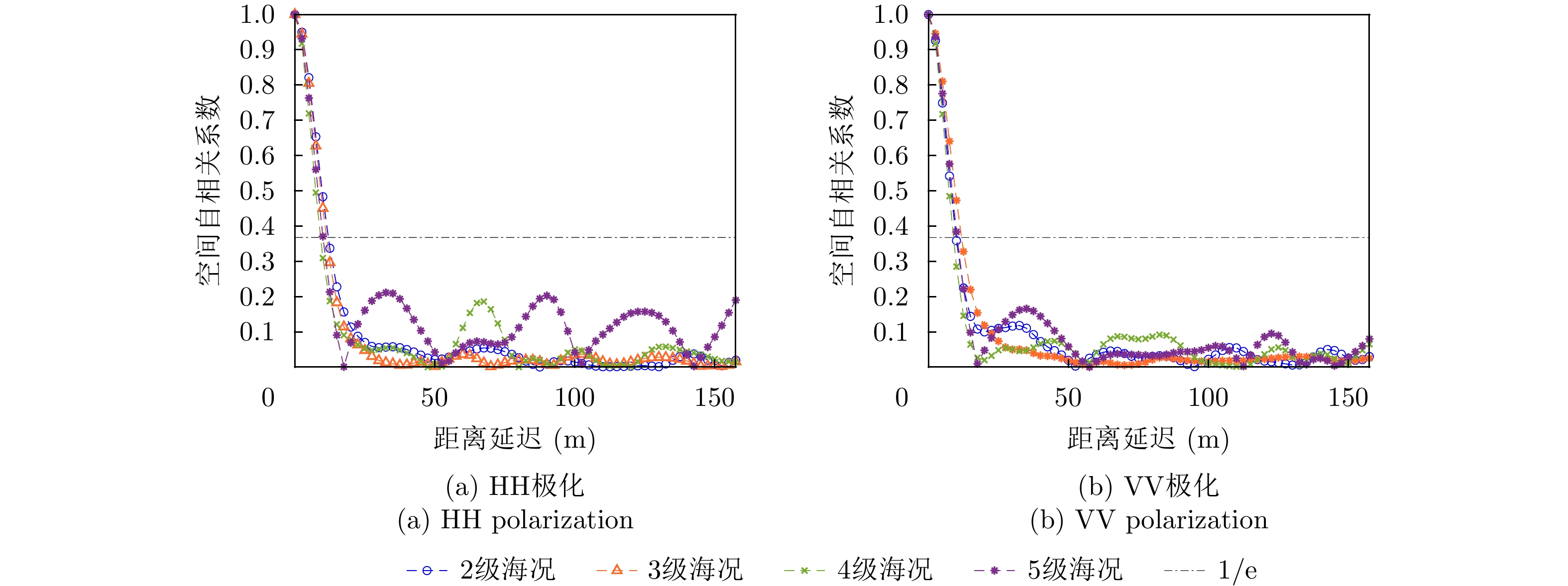
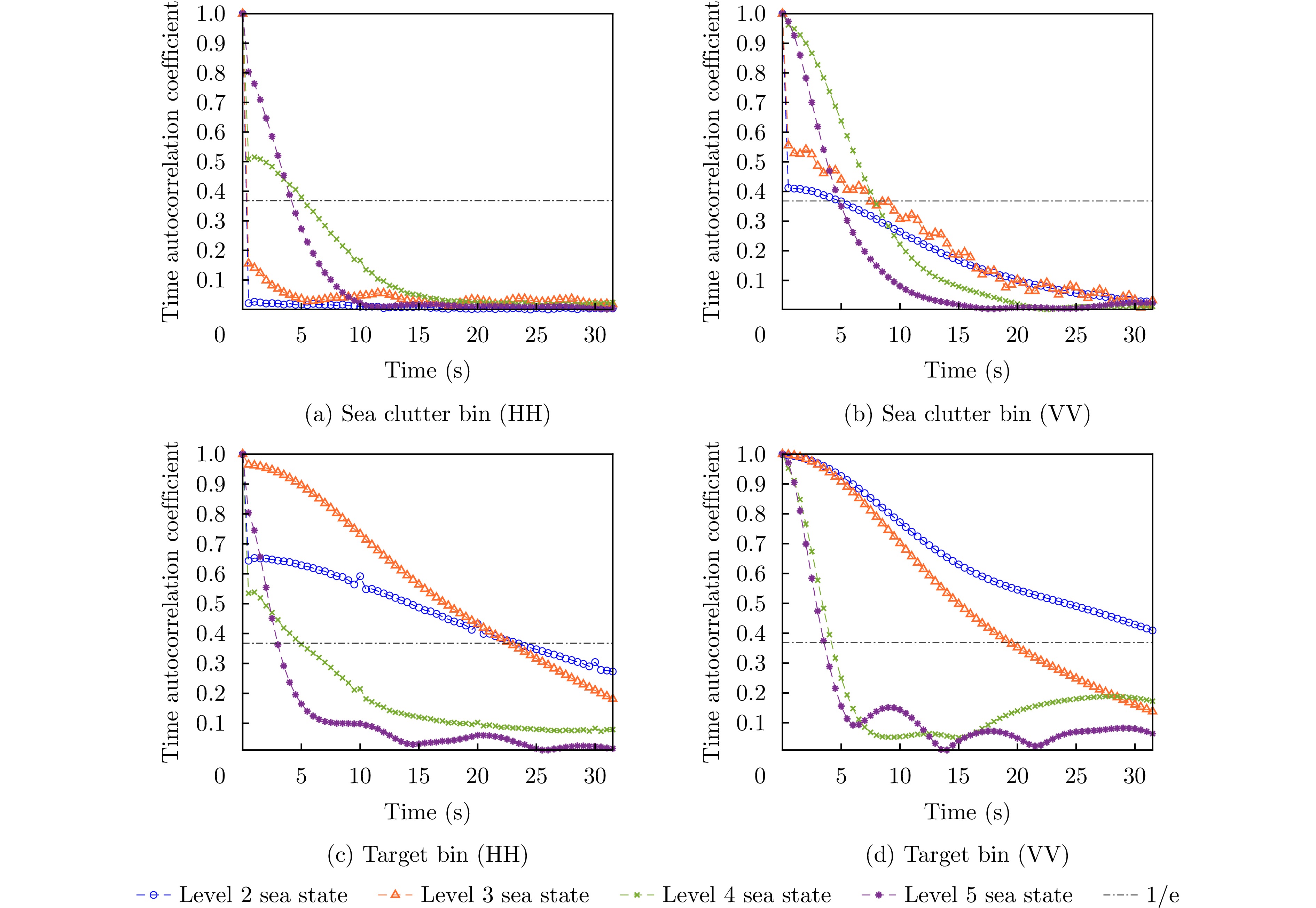
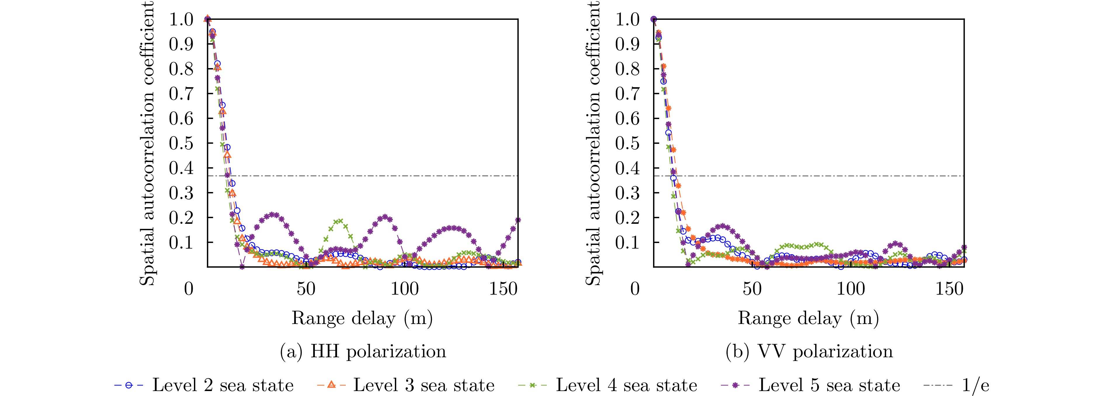
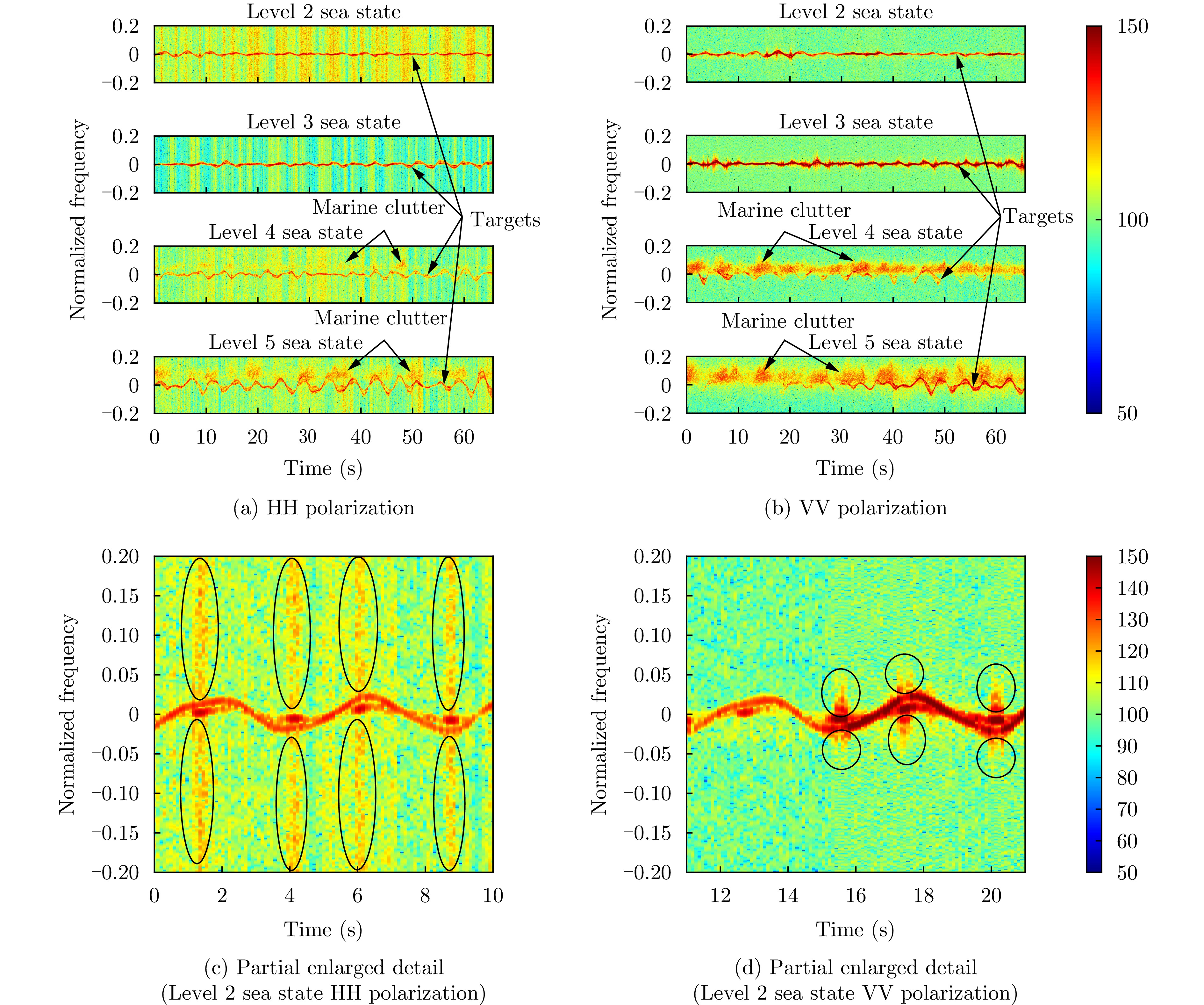
摘要: 海上目标检测识别受制于海上目标及海杂波环境特性,基于实测数据认知海上目标的本质特征有利于推进目标检测识别技术进步。针对海上目标散射特性数据不足的问题,升级“雷达对海探测数据共享计划(SDRDSP)”,扩展雷达目标观测的物理维度、提升雷达及辅助数据采集能力,获取不同极化、海况下的海上目标及环境数据,构建海上目标双极化多海况散射特性数据集,并分析其统计分布特性、时间与空间相关性和多普勒谱特性,为数据使用提供支持。后续将推进海上目标类型与数量的持续积累,为海上目标检测识别性能提升和智能化发展提供数据支持。Abstract: Marine target detection and recognition depend on the characteristics of marine targets and sea clutter. Therefore, understanding the essential features of marine targets based on the measured data is crucial for advancing target detection and recognition technology. To address the issue of insufficient data on the scattering characteristics of marine targets, the Sea-Detecting Radar Data-Sharing Program (SDRDSP) was upgraded to obtain data on marine targets and their environment under different polarizations and sea states. This upgrade expanded the physical dimension of radar target observation and improved radar and auxiliary data acquisition capabilities. Furthermore, a dual-polarized multistate scattering characteristic dataset of marine targets was constructed, and the statistical distribution characteristics, time and space correlation, and Doppler spectrum were analyzed, supporting the data usage. In the future, the types and quantities of maritime targets will continue to accumulate, providing data support for improving marine target detection and recognition performance and intelligence.
-
Key words:
- Radar experiment /
- Sea target detection /
- Sea clutter /
- Target detection and recognition
-
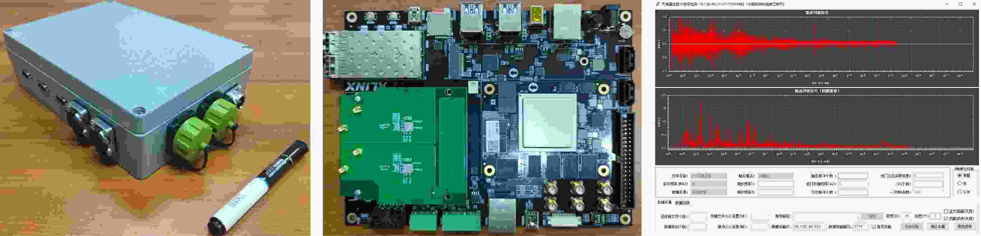
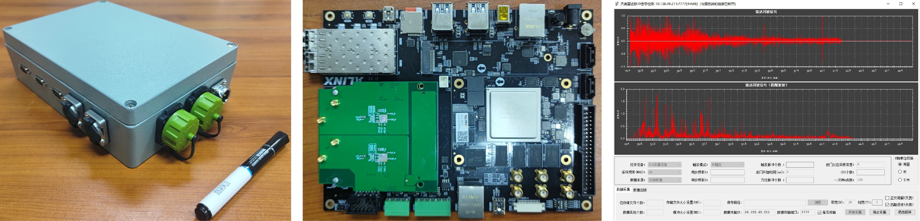
图 3 HD-LD-CJ-22型雷达数据采集设备与显控软件
Figure 3. HD-LD-CJ-22 radar data acquisition and control software

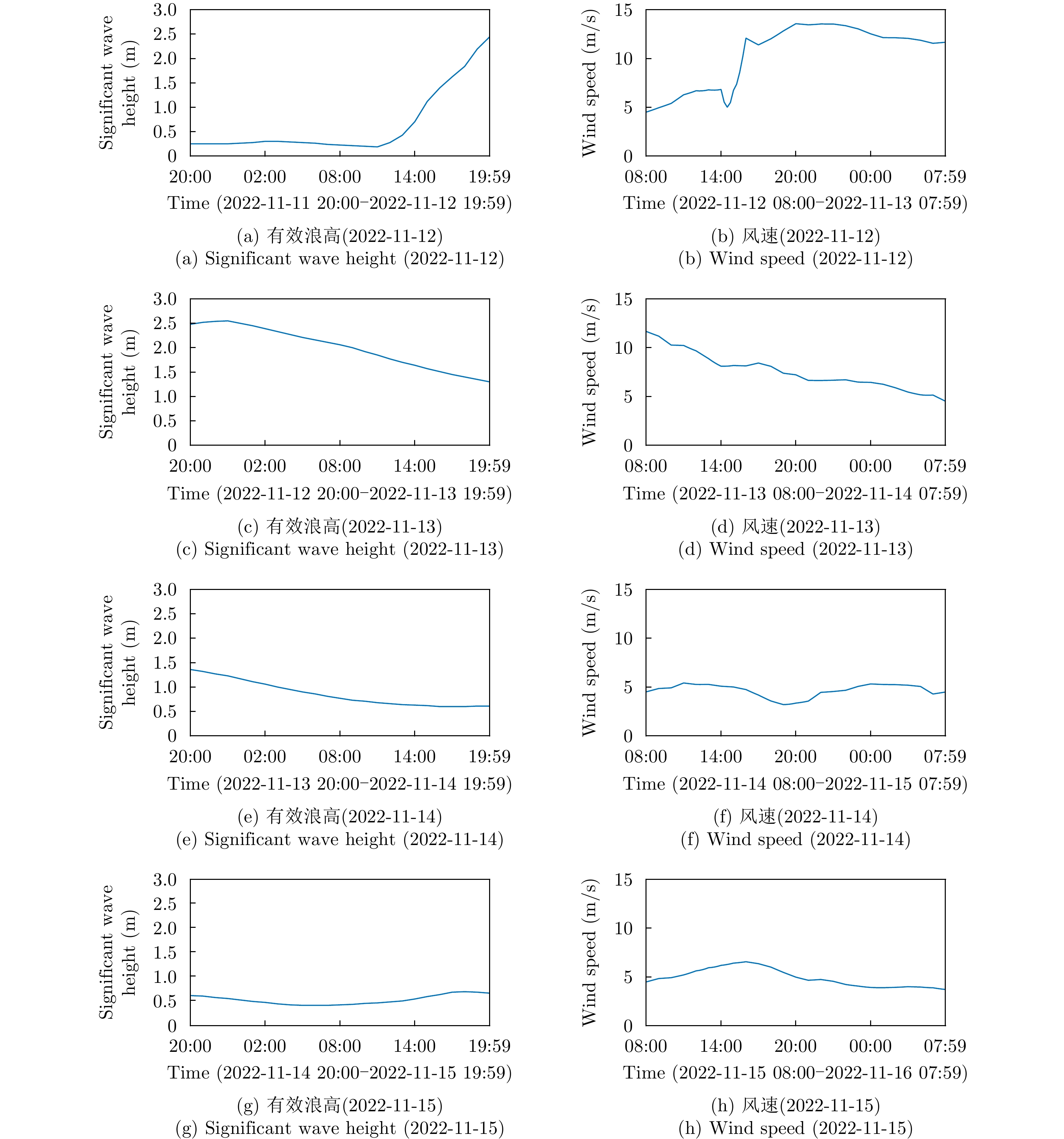
图 6 试验海域气象水文数据(NC数据)
Figure 6. Meteorological and hydrological data of the test sea area (NC data)
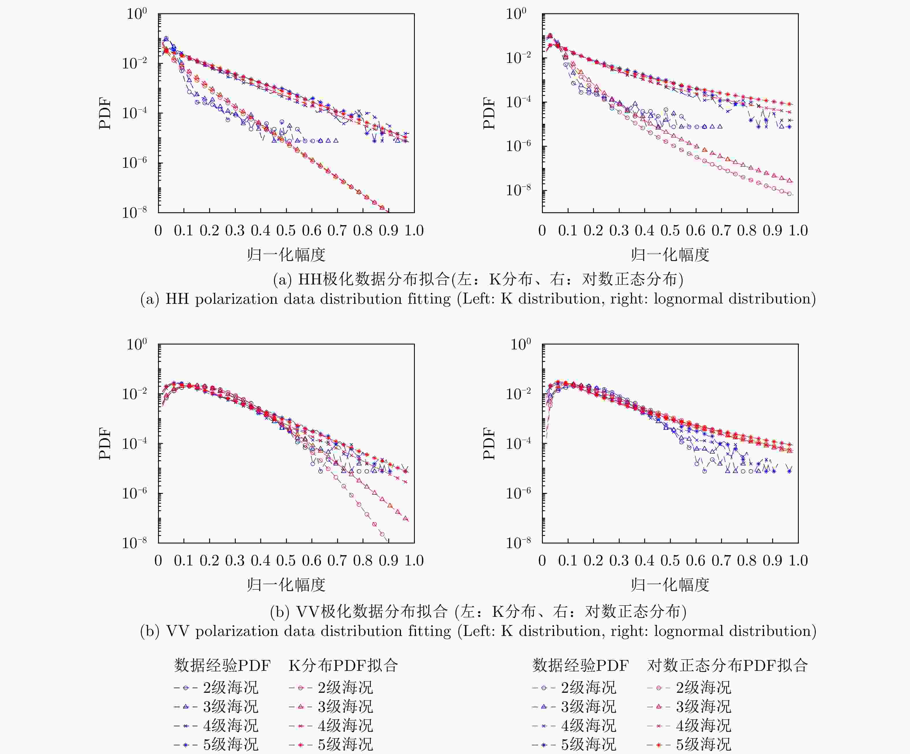
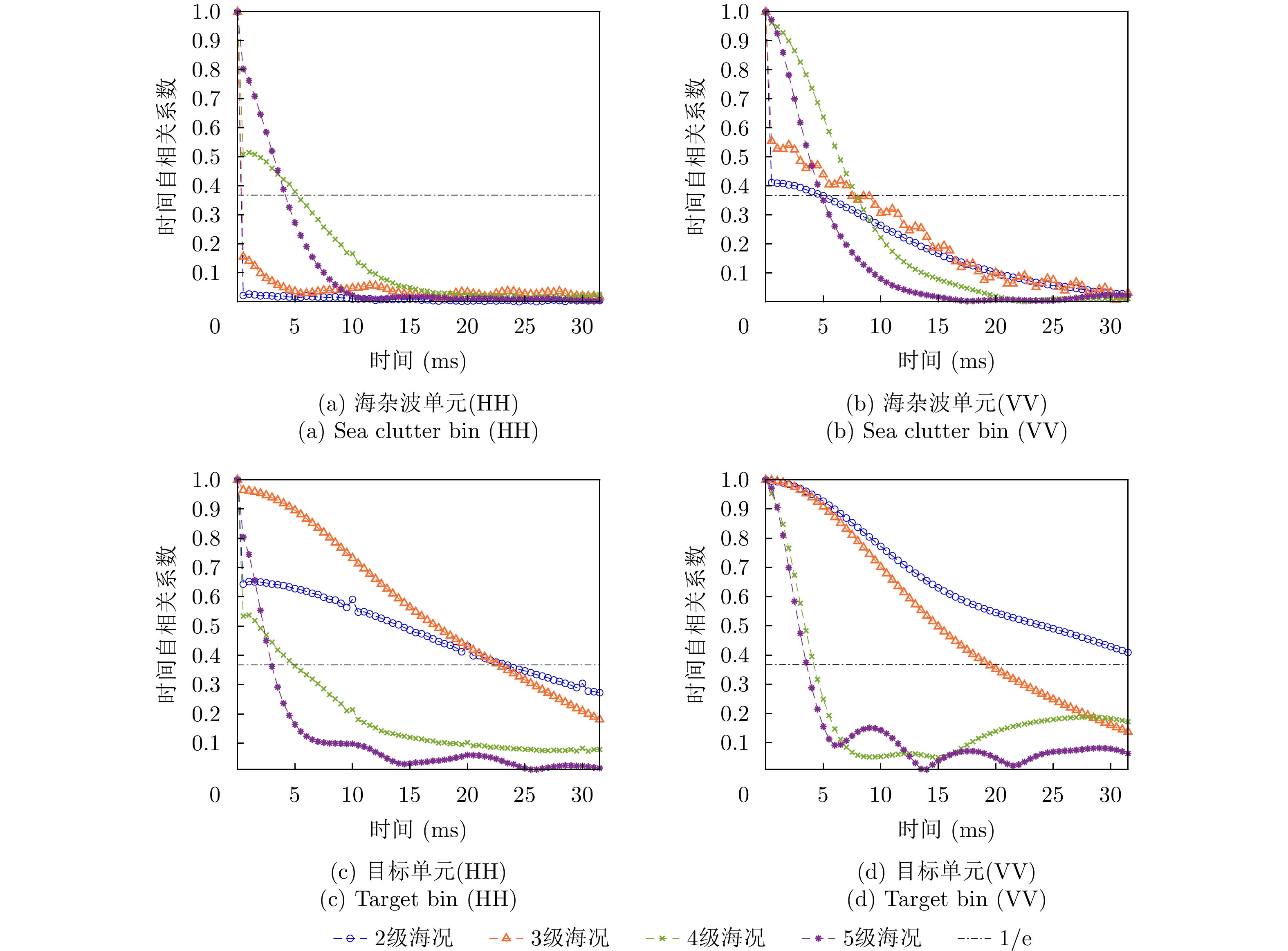
图 9 海杂波单元幅度分布拟合结果
Figure 9. Amplitude distribution fitting results of sea clutter bins
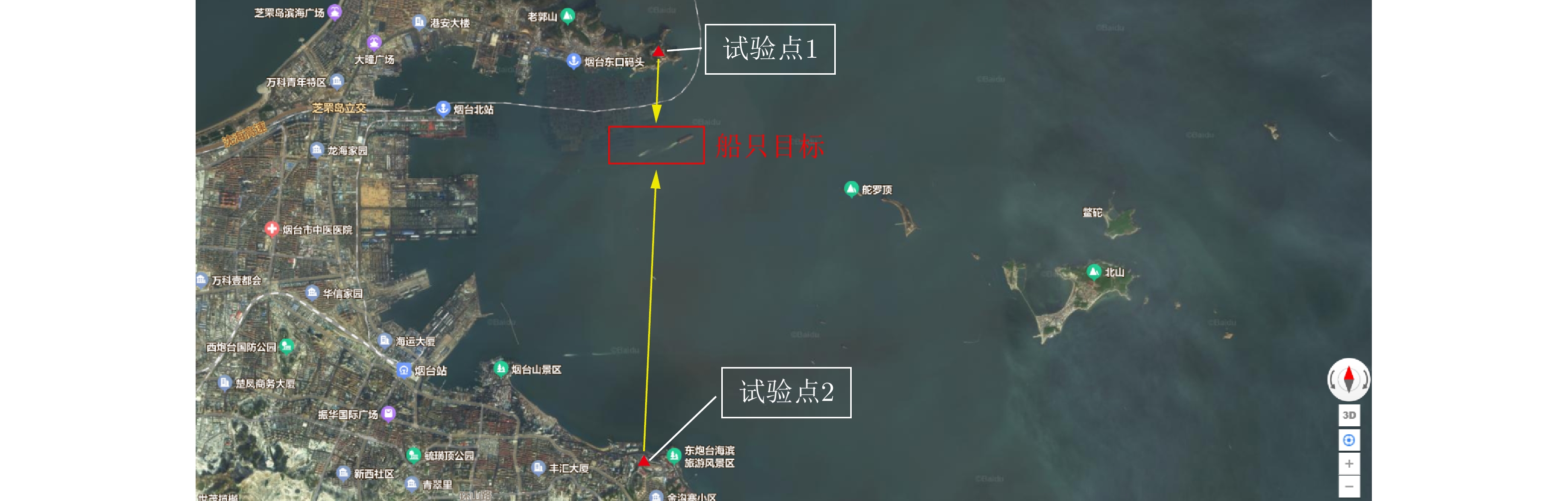
S1 雷达对海探测数据2022年第1期——海上目标散射特性数据集
S1. Sea-detecting radar data 2022 phase 1--Sea target scattering feature dataset
表 1 已共享的雷达对海探测数据
Table 1. Shared sea-detecting radar data
年期 雷达波段 极化方式 数据简介 2019年第1期 X HH 3组数据,主要为扫描和凝视观测模式下的海杂波数据,目标为海面非合作目标。 2020年第1期 X HH 2组数据,主要为凝视观测模式下的海杂波数据、海杂波+目标数据,目标为锚泊船只和航道浮标。 2020年第2期 X HH 2组数据,为海面机动目标跟踪试验数据,目标为海面合作目标(小型快艇)。 2020年第3期 X HH 1组数据,为雷达目标RCS定标试验数据,目标为RCS为0.25 m2不锈钢球,由渔船拖动或漂浮。 2021年第1期 X HH 5组数据,为云雨气象条件下的雷达不同转速扫描试验数据,海面无合作目标。  下载: 导出CSV
表 2 X波段试验雷达参数
Table 2. Parameters of X-band experimental radars
雷达技术指标 HH极化 VV极化 工作频段 X X 工作频率范围 9.3~9.5 GHz 9.3~9.5 GHz 量程 1/16~96 n mile 1/16~96 n mile 扫描带宽 25 MHz (T2, T3) 25 MHz (T2, T3) 距离分辨率 6 m 6 m 脉冲重复频率(kHz) 1.6, 2.0, 3.0, 5.0, 10.0 1.6, 2.0, 3.0, 5.0, 10.0 发射波形 T1:单频
T2:LFM
T3:LFMT1:单频
T2:LFM
T3:LFM脉冲宽度 T1:0.15 μs
T2:8 μs
T3:25 μsT1:0.15 μs
T2:8 μs
T3:25 μs发射峰值功率 100 W 100 W 天线转速(r/min) 2, 6, 12, 24, 48 2, 6, 12, 24, 48 天线长度 2.0 m 2.5 m 天线工作模式 圆扫、扇扫、
固定指向圆扫、扇扫、
固定指向天线极化方式 HH VV 天线水平波束宽度 1.2° 1.1° 天线垂直波束宽度 22° 23°
下载: 导出CSV
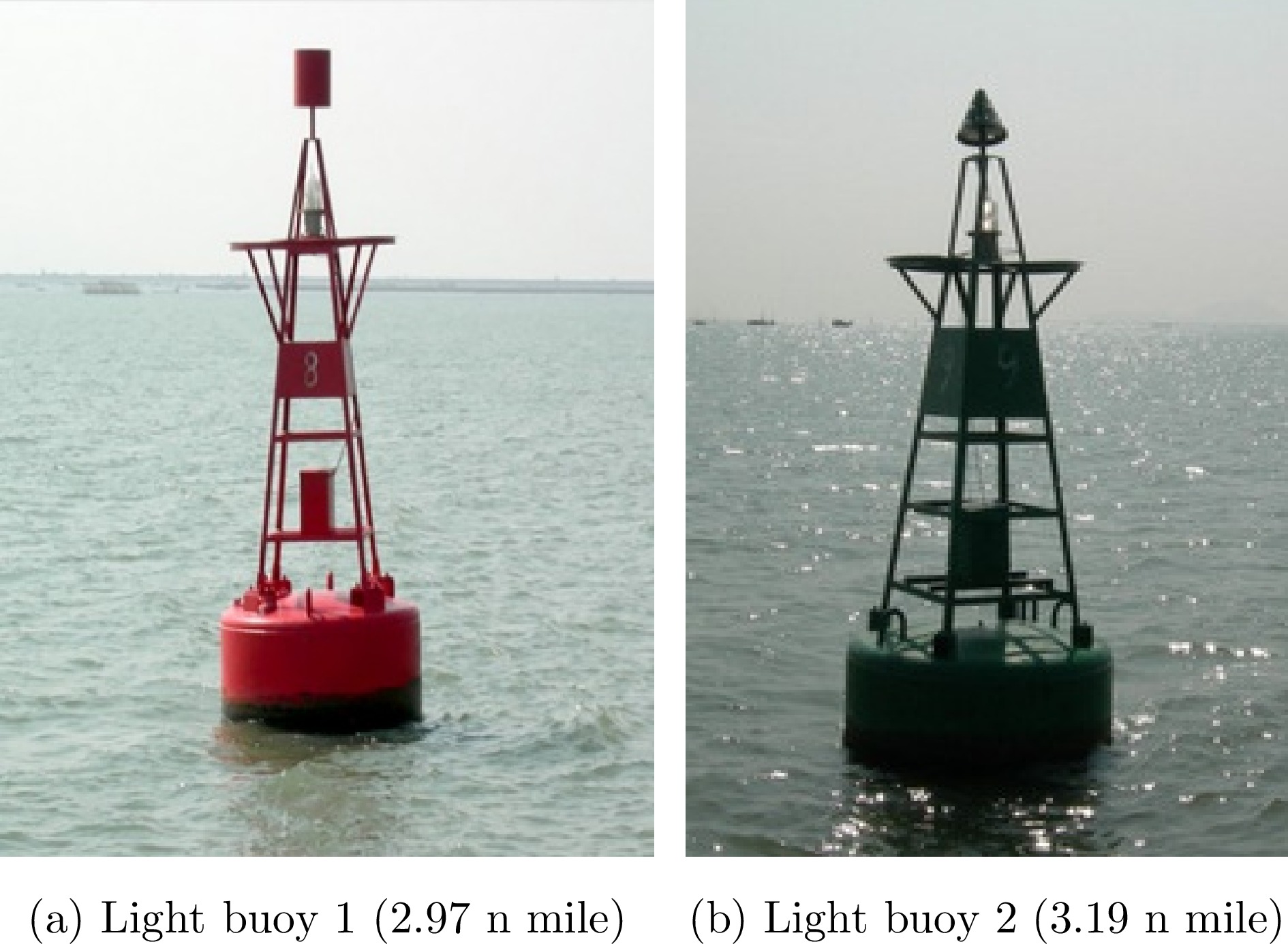
表 3 海上目标散射特性数据集概况表
Table 3. Summary table of sea target scattering characteristics dataset
序号 海况
等级数据
组数雷达天线
工作模式工作
量程发射脉冲模式 目标
种类气象水文数据 擦地角
(°)1 2级 10组 凝视 6 n mile T1+T2 航道浮标 有 0.68~1.09 2 3级 54组 凝视 6 n mile T1+T2 航道浮标 有 0.68~1.09 3 4级 48组 凝视 6 n mile T1+T2 航道浮标 有 0.68~1.09 4 5级 30组 凝视 6 n mile T1+T2 航道浮标 有 0.68~1.09 注:① 每天气象水文数据形成一个nc格式文件,提供风速/风向/浪高/浪向/浪周期信息;
② 凝视模式下每组数据包含的脉冲数均为217个;
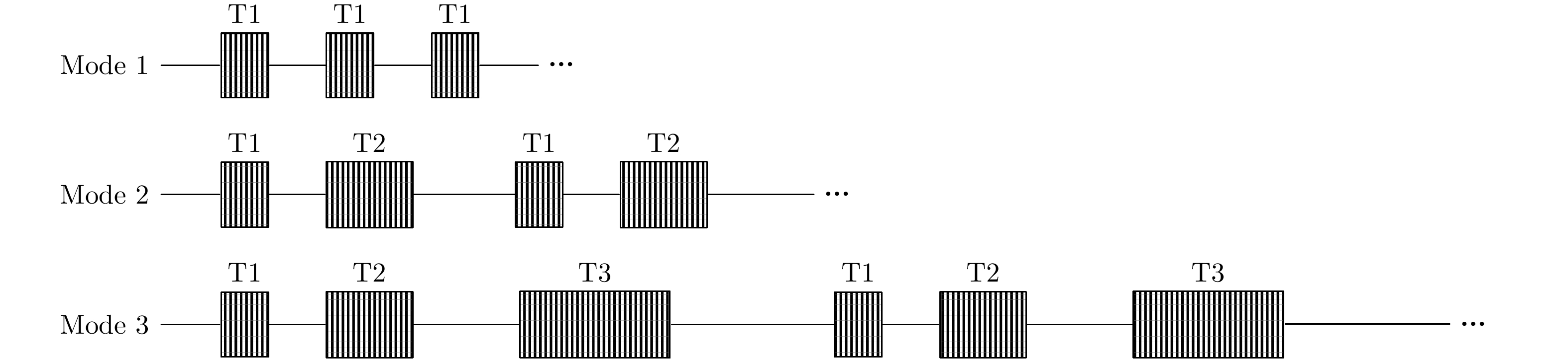
③ 发射脉冲模式T1+T2,对应图2中的模式2;
④ 雷达垂直波束保持不变,擦地角范围是通过雷达架高和数据对应的径向距离范围折算得到的。
下载: 导出CSV
表 4 2-5级海况HH与VV极化雷达示例数据
Table 4. Sample data of HH and VV polarized radars in level 2-5 sea states
数据名 包含
脉冲数PRF
(kHz)T1
采样点数T2
采样点数T1, T2采样起始
距离(km)采样间隔(m) 目标 浪高
(m)浪向 海况
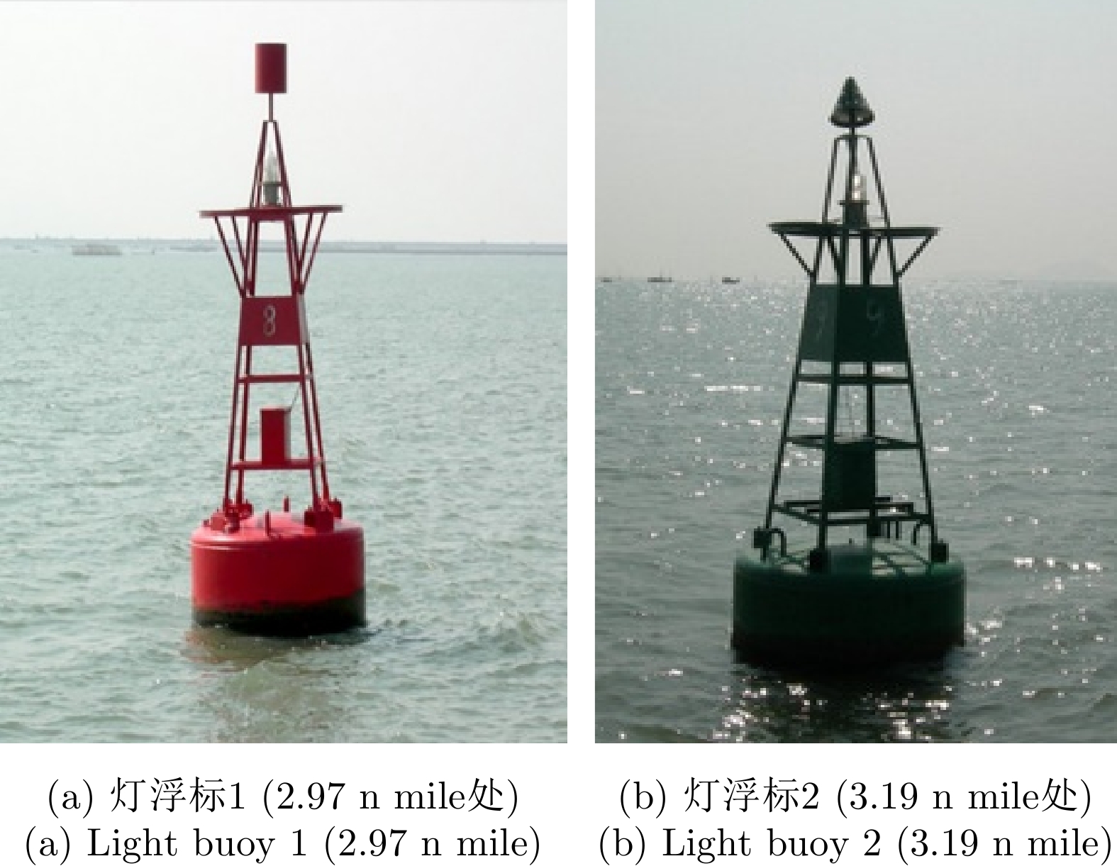
等级20221115050027 _stare_HH217 2 950 1000 4.2525 2.5 浮标1, 2 0.4 西 2级 20221115050036 _stare_VV217 2 950 1000 4.2525 2.5 浮标1, 2 0.4 西 2级 20221114190046 _stare_HH217 2 950 1000 4.2525 2.5 浮标1, 2 0.7 西西北 3级 20221114190055 _stare_VV217 2 950 1000 4.2525 2.5 浮标1, 2 0.7 西西北 3级 20221113210051 _stare_HH217 2 950 1000 4.2525 2.5 浮标1, 2 1.3 北东北 4级 20221113210023 _stare_VV217 2 950 1000 4.2525 2.5 浮标2 1.3 北东北 4级 20221113040027 _stare_HH217 2 950 1000 4.2525 2.5 浮标1, 2 2.6 北 5级 20221113040009 _stare_VV217 2 950 1000 4.2525 2.5 浮标1, 2 2.6 北 5级
下载: 导出CSV
表 1 Shared sea-detecting radar data
Year, issue Radar band Polarization mode Data description 2019, Issue 1 X HH 3 datasets: Primarily sea clutter data collected in scanning and staring observation modes with noncooperative surface targets. 2020, Issue 1 X HH 2 datasets: Sea clutter data and combined sea clutter + target data collected in staring observation mode with anchored vessels and channel buoys as targets. 2020, Issue 2 X HH 2 datasets: Test data for tracking maneuvering surface targets collected using cooperative targets (small speedboats). 2020, Issue 3 X HH 1 dataset: Radar target RCS calibration test data collected using a 0.25 m 2 stainless steel sphere as the target, either towed by a fishing boat or left floating. 2021, Issue 1 X HH 5 datasets: Radar scanning test data under cloudy and rainy meteorological conditions without cooperative surface targets.
下载: 导出CSV
表 2 Parameters of X-band experimental radars
Radar specifications HH polarization VV polarization Operating band X X Operating frequency range (GHz) 9.3–9.5 9.3–9.5 Range (n miles) 1/16–96 1/16–96 Scanning bandwidth (MHz) 25 (T2, T3) 25 (T2, T3) Range resolution (m) 6 6 Pulse repetition frequency (kHz) 1.6, 2.0, 3.0, 5.0, 10.0 1.6, 2.0, 3.0, 5.0, 10.0 Transmit waveform T1:Single frequency
T2:LFM
T3:LFMT1:Single frequency
T2:LFM
T3:LFMPulse width (μs) T1:0.15
T2:8
T3:25T1:0.15
T2:8
T3:25Peak transmit power (W) 100 100 Antenna rotation speed (rpm) 2, 6, 12, 24, 48 2, 6, 12, 24, 48 Antenna length (m) 2.0 2.5 Antenna operating modes Circular, Sector, Fixed Direction Circular, Sector, Fixed Direction Antenna polarization HH VV Antenna horizontal beamwidth (°) 1.2 1.1 Antenna vertical beamwidth (°) 22 23
下载: 导出CSV
表 3 Summary of the datasets of sea target scattering characteristics
No. Marine state level Number of datasets Radar antenna mode Operating range Transmit pulse mode Target type Meteorological and hydrological data Clutter grazing angle (°) 1 Level 2 10 Staring 6 n miles T1+T2 Channel buoy Yes 0.68~1.09 2 Level 3 54 Staring 6 n miles T1+T2 Channel buoy Yes 0.68~1.09 3 Level 4 48 Staring 6 n miles T1+T2 Channel buoy Yes 0.68~1.09 4 Level 5 30 Staring 6 n miles T1+T2 Channel buoy Yes 0.68~1.09 Notes:① Meteorological and hydrological data for each day are stored in a .nc format file, providing information on wind speed, wind direction, wave height, wave direction, and wave period.
② Each dataset in staring mode contains 2 17 pulses.
③ The transmit pulse mode T1 + T2 corresponds to mode 2 in Fig. 2.
④ The radar’s vertical beamwidth remains constant, and the grazing angle range is calculated based on the radar’s installation height and the corresponding radial distance range of the data.
下载: 导出CSV
表 4 Sample data of HH and VV polarized radars in levels 2–5 sea state
Data name Pulse
countPRF
(kHz)T1
sampling
pointsT2
sampling
pointsT1, T2
sampling start
distance (km)Sampling
interval (m)Target Wave
height (m)Wave
directionMarine
state level20221115050027
_stare_HH2 17 2 950 1000 4.2525 2.5 Buoys 1, 2 0.4 West Level 2 20221115050036
_stare_VV2 17 2 950 1000 4.2525 2.5 Buoys 1, 2 0.4 West Level 2 20221114190046
_stare_HH2 17 2 950 1000 4.2525 2.5 Buoys 1, 2 0.7 West-northwest Level 3 20221114190055
_stare_VV2 17 2 950 1000 4.2525 2.5 Buoys 1, 2 0.7 West-northwest Level 3 20221113210051
_stare_HH2 17 2 950 1000 4.2525 2.5 Buoys 1, 2 1.3 North-northeast Level 4 20221113210023
_stare_VV2 17 2 950 1000 4.2525 2.5 Buoy 2 1.3 North-northeast Level 4 20221113040027
_stare_HH2 17 2 950 1000 4.2525 2.5 Buoys 1, 2 2.6 North Level 5 20221113040009
_stare_VV2 17 2 950 1000 4.2525 2.5 Buoys 1, 2 2.6 North Level 5
下载: 导出CSV
-
[1] 关键. 雷达海上目标特性综述[J]. 雷达学报, 2020, 9(4): 674–683. doi: 10.12000/JR20114.GUAN Jian. Summary of marine radar target characteristics[J]. Journal of Radars, 2020, 9(4): 674–683. doi: 10.12000/JR20114. [2] 丁昊, 刘宁波, 董云龙, 等. 雷达海杂波测量试验回顾与展望[J]. 雷达学报, 2019, 8(3): 281–302. doi: 10.12000/JR19006.DING Hao, LIU Ningbo, DONG Yunlong, et al. Overview and prospects of radar sea clutter measurement experiments[J]. Journal of Radars, 2019, 8(3): 281–302. doi: 10.12000/JR19006. [3] 陈小龙, 黄勇, 关键, 等. MIMO雷达微弱目标长时积累技术综述[J]. 信号处理, 2020, 36(12): 1947–1964. doi: 10.16798/j.issn.1003-0530.2020.12.001.CHEN Xiaolong, HUANG Yong, GUAN Jian, et al. Review of long-time integration techniques for weak targets using MIMO radar[J]. Journal of Signal Processing, 2020, 36(12): 1947–1964. doi: 10.16798/j.issn.1003-0530.2020.12.001. [4] 许述文, 白晓惠, 郭子薰, 等. 海杂波背景下雷达目标特征检测方法的现状与展望[J]. 雷达学报, 2020, 9(4): 684–714. doi: 10.12000/JR20084.XU Shuwen, BAI Xiaohui, GUO Zixun, et al. Status and prospects of feature-based detection methods for floating targets on the sea surface[J]. Journal of Radars, 2020, 9(4): 684–714. doi: 10.12000/JR20084. [5] 贺丰收, 何友, 刘准钆, 等. 卷积神经网络在雷达自动目标识别中的研究进展[J]. 电子与信息学报, 2020, 42(1): 119–131. doi: 10.11999/JEIT180899.HE Fengshou, HE You, LIU Zhunga, et al. Research and development on applications of convolutional neural networks of radar automatic target recognition[J]. Journal of Electronics &Information Technology, 2020, 42(1): 119–131. doi: 10.11999/JEIT180899. [6] 刘宁波, 董云龙, 王国庆, 等. X波段雷达对海探测试验与数据获取[J]. 雷达学报, 2019, 8(5): 656–667. doi: 10.12000/JR19089.LIU Ningbo, DONG Yunlong, WANG Guoqing, et al. Sea-detecting X-band radar and data acquisition program[J]. Journal of Radars, 2019, 8(5): 656–667. doi: 10.12000/JR19089. [7] 刘宁波, 丁昊, 黄勇, 等. X波段雷达对海探测试验与数据获取年度进展[J]. 雷达学报, 2021, 10(1): 173–182. doi: 10.12000/JR21011.LIU Ningbo, DING Hao, HUANG Yong, et al. Annual progress of the sea-detecting X-band radar and data acquisition program[J]. Journal of Radars, 2021, 10(1): 173–182. doi: 10.12000/JR21011. [8] DROSOPOULOS A. Description of the OHGR database[R]. Technical Note 94–14, 1994. [9] DE WIND H J, CILLIERS J C, and HERSELMAN P L. DataWare: Sea clutter and small boat radar reflectivity databases [Best of the Web][J]. IEEE Signal Processing Magazine, 2010, 27(2): 145–148. doi: 10.1109/msp.2009.935415. -


计量
- 文章访问数:
- HTML全文浏览量:
- PDF下载量:
- 被引次数: 0

