无先验模型复杂结构设施SAR全方位三维成像方法研究

林赟; 张琳; 韦立登; 张汉卿; 冯珊珊; 王彦平; 洪文

doi:10.12000/JR22148

无先验模型复杂结构设施SAR全方位三维成像方法研究

DOI: 10.12000/JR22148

林赟¹,
张琳¹,
韦立登²,
张汉卿^{3, 4},
冯珊珊^{3, 4},
王彦平¹,
洪文^{3, 4, ,}

1.
北方工业大学信息学院雷达监测技术实验室北京 100144
2.
北京无线电测量研究所北京 100854
3.
中国科学院空天信息创新研究院北京 100094
4.
中国科学院空间信息处理与应用系统技术重点实验室北京 100190

基金项目: 国家自然科学基金(61860206013, 62131001)，快速扶持项目(80913010302)，北京市教育委员会创新团队建设计划(IDHT20190501)

详细信息

作者简介:
林　赟，博士，副研究员，硕士生导师，主要研究方向为多角度SAR三维成像技术

韦立登，博士，研究员，研究方向为机载SAR成像与InSAR处理技术

洪　文，博士，研究员，博士生导师，研究方向为合成孔径雷达(SAR)成像新概念新体制、多维度SAR成像机理与方法

通讯作者:
洪文 whong@mail.ie.ac.cn

责任主编：张晓玲 Corresponding Editor: ZHANG Xiaoling
中图分类号: TN959
计量
- 文章访问数: 1290
- HTML全文浏览量: 647
- PDF下载量: 231
- 被引次数: 10
出版历程
- 收稿日期: 2022-07-14
- 修回日期: 2022-08-04
- 网络出版日期: 2022-08-22
- 刊出日期: 2022-10-28

Research on Full-aspect Three-dimensional SAR Imaging Method for Complex Structural Facilities without Prior Model

LIN Yun¹,
ZHANG Lin¹,
WEI Lideng²,
ZHANG Hanqing^{3, 4},
FENG Shanshan^{3, 4},
WANG Yanping¹,
HONG Wen^{3, 4
, ,}

1.
Radar Monitoring Technology Laboratory, School of Information, North China University of Technology, Beijing 100144, China
2.
Beijing Institute of Radio Measurement, Beijing 100854, China
3.
Aerospace Information Research Institute, Chinese Academy of Sciences, Beijing 100094, China
4.
Key Laboratory of Technology in Geo-Spatial Information Processing and Application System, Chinese Academy of Sciences, Beijing 100190, China

Funds: The National Natural Science Foundation of China (61860206013, 62131001), Rapid Support Project (80913010302), Innovation Team Building Support Program of Beijing Municipal Education Commission (IDHT20190501)

More Information

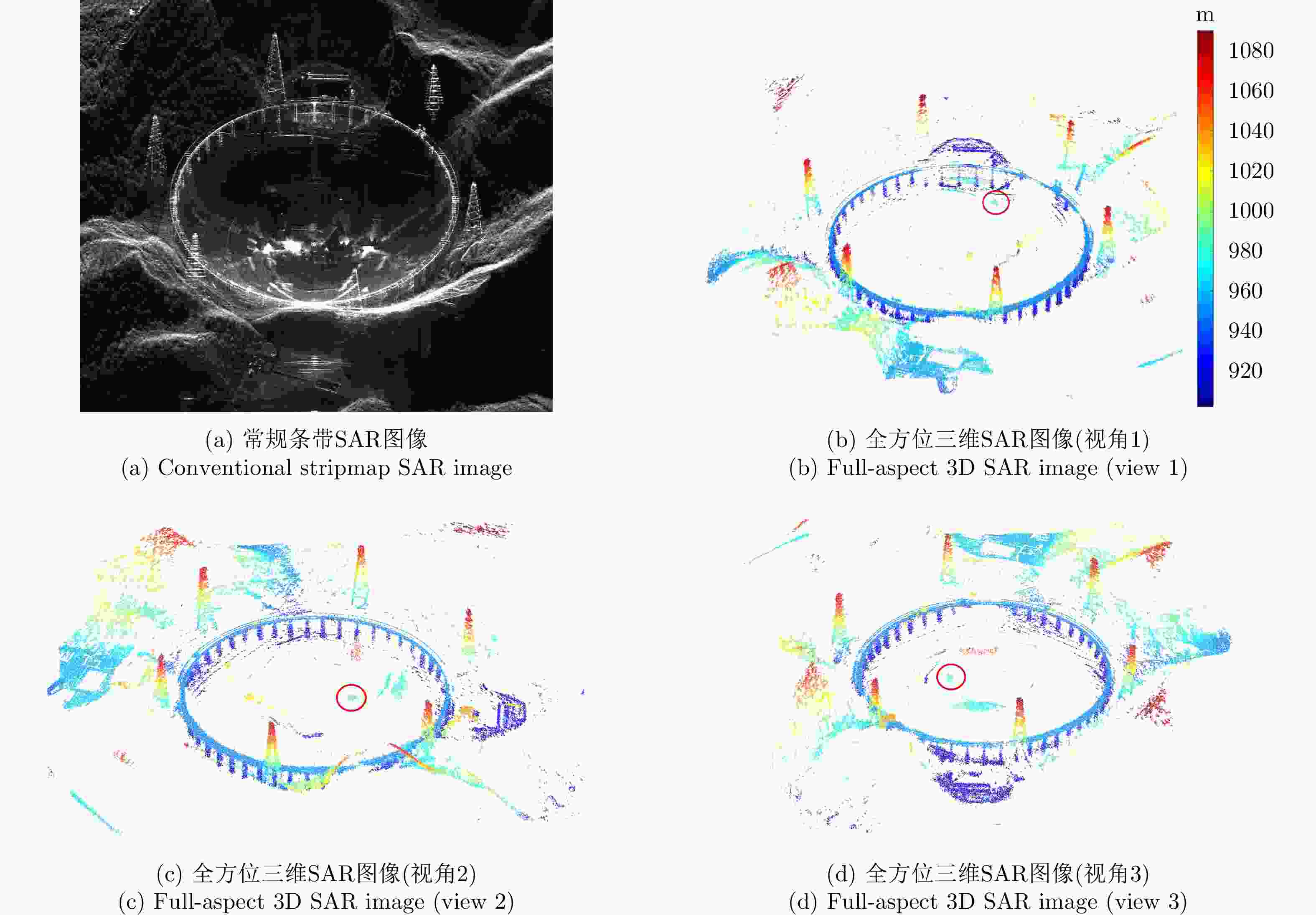
Corresponding author: HONG Wen, whong@mail.ie.ac.cn

摘要

摘要: 复杂结构设施的SAR三维成像是SAR成像领域的热点和难点问题。现有SAR三维成像依赖于高程方向的多通道或多次飞行，对雷达系统或数据获取的要求较高。该文提出无先验模型复杂结构设施三维成像方法，仅需一次飞行即可获得先验信息未知区域全场景全方位三维图像。该方法充分利用圆迹SAR的全方位观测、解叠掩和解高程模糊优势，无需目标预先建模和三维成像网格构建，适用于大面积区域复杂结构设施的精细三维成像，在雷达三维成像实用化技术方面取得了重要进展。通过该方法首次获得FAST射电望远镜的雷达全方位三维图像，验证了理论与方法的正确性与有效性。
- SAR三维成像 /
- 多角度SAR /
- 全方位SAR /
- 圆迹SAR /
- 干涉SAR
Abstract: SAR three-Dimensional (3D) imaging of complex structural facilities is an important and challenging issue in SAR imaging. The existing 3D SAR imaging relies on multiple channels or flights in the elevation direction, exerting high demands on the radar system or data acquisition. This paper proposes a 3D imaging method for complex structural facilities without a prior model, and the full-aspect 3D image of the entire scene in the region with unknown prior information can be obtained solely using a single flight. This method completely utilizes the full-aspect observation as well as the layover and elevation ambiguity resolving capabilities of circular SAR without requiring target pre-modeling and 3D imaging grid construction. Moreover, the method is suitable for fine 3D imaging complex structural facilities in large areas. Significant progress has been made in the practical technology of radar 3D imaging. The full-aspect 3D radar images of the FAST radio telescope are obtained for the first time with the proposed method, thus verifying the correctness and effectiveness of our theory and method.
- 3D SAR imaging /
- Multi-aspect SAR /
- Full-aspect SAR /
- Circular SAR /
- InSAR

HTML全文

1. Introduction

In recent years, Frequency Diverse Array (FDA) radar has received much attention due to its range-angle-time-dependent beampattern^[1,2]. Combining the advantages of FDA and traditional phased array Multiple-Input Multiple-Output (MIMO) radar in the degree of freedom, the FDA Multiple-Input Multiple Output (FDA-MIMO) radar was proposed in Ref. [3] and applied in many fields^[4-9]. For parameter estimation algorithm, the authors first proposed a FDA-MIMO target localization algorithm based on sparse reconstruction theory^[10], and an unbiased joint range and angle estimation method was proposed in Ref. [11]. The work of Ref. [12] further proved that the FDA-MIMO is superior to traditional MIMO radar in range and angle estimation performance, and the authors of Ref. [13] introduced a super-resolution MUSIC algorithm for target location, and analyzed its resolution threshold. Meanwhile, high-resolution Doppler processing is utilized for moving target parameter estimation^[14]. The Estimation of Signal Parameters via Rotational Invariance Technique (ESPRIT) and PARAllel FACtor (PARAFAC) was proposed in Ref. [15], which is a search-free algorithm for FDA-MIMO.

Moreover, the research of conformal array has received more and more attention. Conformal array is a non-planar array that can be completely attached to the surface of the carrier^[16]. It has significant advantages such as reducing the aerodynamic impact on the carrier and smaller radar cross section^[17]. In addition, conformal array can achieve wide-angle scanning with a lower SideLobe Level (SLL)^[18]. Different from traditional arrays, the element beampattern of conformal array needs to be modeled separately in the parameter estimation due to the difference of carrier curvature^[19-21].

As far as we know, most of the existing researches on FDA-MIMO are based on linear array, while there is little research on the combination of FDA-MIMO and conformal array^[22]. In this paper, we replace the receiving array in the traditional FDA-MIMO with conformal array. Compared with conventional FDA-MIMO, conformal FDA-MIMO inherits the merits of conformal array and FDA-MIMO, which can effectively improve the stealth and anti-stealth performance of the carrier, and reduce the volume and the air resistance of the carrier. For conformal FDA-MIMO, we further study the parameters estimation algorithm. The major contributions of this paper are summarized as follows:

(1) A conformal FDA-MIMO radar model is first formulated.

(2) The parameter estimation Cramér-Rao Lower Bound (CRLB) for conformal FDA-MIMO radar is derived.

(3) Inspired by the existing work of Refs. [23,24], a Reduced-Dimension MUSIC (RD-MUSIC) algorithm for conformal FDA-MIMO radar is correspondingly proposed to reduce the complexity.

The rest of the paper consists of four parts. Section 2 formulates the conformal FDA-MIMO radar model, and Section 3 derives a RD-MUSIC algorithm for conformal FDA-MIMO radar. Simulation results for conformal FDA-MIMO radar with semi conical conformal receiving array are provided in Section 4. Finally, conclusions are drawn in Section 5.

2. Conformal FDA-MIMO Radar

2.1 General conformal FDA-MIMO signal model

For the convenience of analysis, we consider a monostatic conformal FDA-MIMO radar which is composed by a $M$ -element linear FDA transmitting array and a $N$ -element conformal receiving array, as shown in Fig. 1. d denotes the inter-element spacing, the carrier frequency at the mth transmitting element is ${f_m} = {f_1} + \Delta f(m - 1)$ , $m = 1,2, \cdots ,M$ where ${f_1}$ is the transmission frequency of the first antenna element, which is called as reference frequency, and $\Delta f$ is the frequency offset between the adjacent array elements.

Figure 1. Conformal FDA-MIMO radar

DownLoad: Full-Size Img PowerPoint

The complex envelope of the transmitted signal of the mth transmitting element is denoted as ${{\varphi _m}} (t)$ , assume the transmitting waveforms have orthogonality,

$\int_{{T_p}} {{\varphi _m}} (t)\varphi _{{m_1}}^*(t - \tau ){\rm{d}}t = 0,\quad {m_1} \ne m$

(1)

where $\tau$ denotes the time delay, ${T_p}$ denotes the pulse duration, and ${\left( \cdot \right)^ * }$ is conjugate operator. The signal transmitted from the mth element can be expressed as

${s_m}(t) = {a_m}(t,\theta ,\phi ,r){\varphi _m}(t),\quad 0 \le t \le {T_p}$

(2)

where

$\begin{split} & {a_m}(t,\theta ,\phi ,r) \hfill \\ & =\exp \left\{ { - {\rm{j}}2\pi \left( \begin{gathered} \frac{{(m - 1)\Delta fr}}{{\rm{c}}} - \frac{{{f_1}(m - 1){{d}}\sin \alpha }}{{\rm{c}}} \hfill \\ - (m - 1)\Delta ft \hfill \\ \end{gathered} \right)} \right\} \end{split}$

(3)

is the mth element of the transmitting steering vector according to the phase difference between adjacent elements, the angle between far-field target and transmitting array is denoted as $\alpha = \arcsin (\sin \theta \cos \phi )$ , where $\arcsin ( \cdot )$ denotes arcsine operator, $\alpha$ can be calculated by using the inner product between the target vector and unit vector along the $X$ -axis. $\theta ,\phi ,r$ are the elevation, azimuth and range between the target and the origin point, respectively. The phase difference between adjacent elements is

$\Delta {\psi _{t0}} = 2\pi \left( {\frac{{\Delta fr}}{{\rm{c}}} - \frac{{{f_1}d\sin \alpha }}{{\rm{c}}} - \Delta ft} \right)$

(4)

where ${\rm{c}}$ is light speed. For far-field target ${P}\left( {r,\theta ,\phi } \right)$ , the transmitting steering vector is

$\begin{split} {{\boldsymbol{a}}_0}\left( {t,\theta ,\phi ,r} \right) =& \left[ {1,\exp \left\{ { - {\rm{j}}\Delta {\psi _{t0}}} \right\}, \cdots ,} \right. \\ &{\left. {\exp \left\{ { - {\rm{j}}(M - 1)\Delta {\psi _{t0}}} \right\}} \right]^{\rm{T}}} \end{split}$

(5)

For the conformal receiving array, as shown in Fig. 1(b), the time delay between target ${P}\left( {r,\theta ,\phi } \right)$ and the nth receiving array element is

${\tau _n} = {r_n}/{\rm{c}}$

(6)

where ${r_n}$ is the range between target and the nth receiving array element. For far-field assumption, the ${r_n}$ can be approximated as

${r_n} \approx r - {\vec {\boldsymbol{p}}_n} \cdot \vec {\boldsymbol{r}}$

(7)

where r denotes the range between the target and the origin point, ${\vec {\boldsymbol{p}}_n} = {x_n}{{\boldsymbol{e}}_x} + {y_n}{{\boldsymbol{e}}_y} + {z_n}{{\boldsymbol{e}}_z}$ denotes the position vector from the nth element to origin point, and $\vec {\boldsymbol{r}} = \sin \theta \cos \phi {{\boldsymbol{e}}_x} + \sin \theta \sin \phi {{\boldsymbol{e}}_y} + \cos\theta {{\boldsymbol{e}}_z}$ is the unit vector in target orientation, where ${{\boldsymbol{e}}_x},{{\boldsymbol{e}}_y}$ and ${{\boldsymbol{e}}_z}$ are the unit vectors along the X- , Y- , and $Z$ -axis, respectively. $({x_n},{y_n},{z_n})$ are the coordinates of the nth element in the Cartesian coordinate system. For simplicity, we let $u = \sin \theta \cos \phi$ , $v = \sin \theta \cos \phi$ , so the time delay ${\tau _n} =$ $(r - (u{x_n} + v{y_n} + \cos \theta {z_n}))/{\rm{c}}$ . The time delay between the first element and the nth element at the receiving array is expressed as

$\begin{split} \Delta {\tau _{{r_n}}} =& {\tau _1} - {\tau _n} \\ =& \frac{{u({x_n} - {x_1}) + v({y_n} - {y_1}) + \cos \theta ({z_n} - {z_1})}}{{\rm{c}}} \\ \end{split}$

(8)

And the corresponding phase difference between the first element and the nth element is

$\Delta {\psi _{{R_n}}} = 2\pi {f_1}\Delta {\tau _{{r_n}}}$

(9)

Consequently, the receiving steering vector is

$\begin{split} {\boldsymbol{b}}\left( {\theta ,\phi } \right) =& \left[ {{r_1}(\theta ,\phi ),{r_2}(\theta ,\phi )\exp (j\Delta {\psi _{{r_2}}}), \cdots ,} \right. \\ &{\left. {{r_N}(\theta ,\phi )\exp({\rm{j}}\Delta {\psi _{{r_N}}})} \right]^{\rm{T}}} \\ \end{split}$

(10)

where ${r_n}(\theta ,\phi )$ is the nth conformal receiving array element beampattern which should be designed in its own local Cartesian coordinate system. In this paper, we utilize Euler rotation method to establish transformation frame between local coordinate system and global coordinate system^[25,26].

Then the total phase difference between adjacent transmitting array elements can be rewritten as

$\Delta {\psi _t} = 2\pi \left( {\frac{{\Delta f2r}}{{\rm{c}}} - \frac{{{f_1}d\sin \alpha }}{{\rm{c}}} - \Delta ft} \right)$

(11)

where the factor $2r$ in the first term represents the two-way transmission and reception, and the correspondingly transmitting steering vector is written as

$\begin{split} {\boldsymbol{a}}\left( {t,\theta ,\phi ,r} \right) =& \left[ {1,\exp \left\{ { - {\rm{j}}\Delta {\psi _t}} \right\}, \cdots ,} \right. \\ & {\left. {\exp \left\{ { - {\rm{j}}(M - 1)\Delta {\psi _t}} \right\}} \right]^{\rm{T}}} \end{split}$

(12)

Assuming L far-field targets are located at $\left( {{\theta _i},{\phi _i},{R_i}} \right)$ , $i = 1,2,\cdots,L$ and snapshot number is $K$ . After matched filtering, the received signal can be formulated as following matrix (13,14)

${\boldsymbol{X = AS + N}}$

(13)

where the array manifold ${\boldsymbol{A}}$ is expressed as

$\begin{split} {\boldsymbol{A}} = &\left[ {{{\boldsymbol{a}}_{t,r}}\left( {{\theta _1},{\phi _1},{r_1}} \right), \cdots ,{{\boldsymbol{a}}_{t,r}}\left( {{\theta _L},{\phi _L},{r_L}} \right)} \right] \hfill \\ =& \left[ {\boldsymbol{b}}\left( {{\theta _1},{\phi _1}} \right) \otimes {\boldsymbol{a}}\left( {{\theta _1},{\phi _1},{r_1}} \right), \cdots ,{\boldsymbol{b}}\left( {{\theta _L},{\phi _L}} \right) \right.\\ & \left.\otimes {\boldsymbol{a}}\left( {{\theta _L},{\phi _L},{r_L}} \right) \right] \end{split}$

(14)

where ${{\boldsymbol{a}}_{t,r}}\left( {\theta ,\phi ,r} \right)$ is the joint transmitting-receiving steering vector, ${\boldsymbol{S}} = \left[ {s({t_1}),s({t_2}), \cdots ,s({t_K})} \right] \in {\mathbb{C}^{L \times K}}$ and ${\boldsymbol{N}} \in {\mathbb{C}^{MN \times K}}$ denote the signal matrix and noise matrix, respectively, where noise follows the independent identical distribution, and $\otimes$ denotes Kronecker product.

$\begin{split} {\boldsymbol{a}}\left( {\theta ,\phi ,r} \right) =& \left[ 1\; {\exp \left\{ { - {\rm{j}}2\pi \left( {\dfrac{{2\Delta fr}}{{\rm{c}}} - \dfrac{{{f_1}d\sin \alpha }}{{\rm{c}}}} \right)} \right\}} \right. \hfill \\ &\left. \cdots {\exp \left\{ { - {\rm{j}}2\pi (M - 1)\left( {\dfrac{{2\Delta fr}}{{\rm{c}}} - \dfrac{{{f_1}d\sin \alpha }}{{\rm{c}}}} \right)} \right\}} \right] \end{split}$

(15)

which can be expressed as

${\boldsymbol{a}}\left( {\theta ,\phi ,r} \right) = {\boldsymbol{a}}\left( {\theta ,\phi } \right) \odot {\boldsymbol{a}}\left( r \right)$

(16)

where

$\begin{split} {\boldsymbol{a}}(r) =& \left[ {1,\exp \left( - {\rm{j}}2\pi \frac{{2\Delta fr}}{{\rm{c}}}\right), \cdots ,} \right. \\ & {\left. {\exp\left( { - {\rm{j}}2\pi (M - 1)\frac{{2\Delta fr}}{{\rm{c}}}} \right)} \right]^{\rm{T}}}\qquad \end{split}$

(17)

$\begin{split} {\boldsymbol{a}}(\theta ,\phi ) =& \left[ {1,\exp \left({\rm{j}}2\pi \frac{{{f_1}d\sin \alpha }}{{\rm{c}}}\right),} \cdots ,\right. \hfill \\ &{\left. { \exp \left[{\rm{j}}2\pi (M - 1)\frac{{{f_1}d\sin \alpha }}{{\rm{c}}}\right]} \right]^{\rm{T}}} \end{split}$

(18)

and $\odot$ represents Hadamard product operator.

2.2 CRLB of conformal FDA-MIMO

The CRLB can be obtained from the inverse of Fisher information matrix^[27,28], which establishes a lower bound for the variance of any unbiased estimator. We employ the CRLB for conformal FDA-MIMO parameter estimation to evaluate the performance of some parameter estimation algorithms.

The discrete signal model is

${\boldsymbol{x}}[k] = {{\boldsymbol{a}}_{t,r}}(\theta ,\phi ,r)s[k] + {\boldsymbol{N}}[k],\quad k = 1,2, \cdots ,K$

(19)

For the sake of simplification, we take ${{\boldsymbol{a}}_{t,r}}$ as the abbreviation of ${{\boldsymbol{a}}_{t,r}}(\theta ,\phi ,r)$ .

The Probability Distribution Function (PDF) of the signal model with $K$ snapshots is

$\begin{split} p({\boldsymbol{x}}\left| {\theta ,\phi ,r} \right.) =& \frac{1}{{{{(2\pi \sigma _n^2)}^{\textstyle\frac{K}{2}}}}} \\ & \cdot \exp \left( - \frac{1}{{\sigma _n^2}}{({\boldsymbol{x}} - {{\boldsymbol{a}}_{t,r}}{\boldsymbol{s}})^{\rm{H}}}({\boldsymbol{x}} - {{\boldsymbol{a}}_{t,r}}{\boldsymbol{s}})\right) \\ \end{split}$

(20)

where ${\boldsymbol{x}} = [{\boldsymbol{x}}(1),{\boldsymbol{x}}(2),\cdots,{\boldsymbol{x}}(K)]$ and ${\boldsymbol{s}} = [s(1),$ $s(2), \cdots,s(K)]$ .

The CRLB matrix form of elevation angle, azimuth angle and range is given by Eq. (21), diagonal elements $\left\{ {{C_{\theta \theta }},{C_{\phi\phi} } ,{C_{rr}}} \right\}$ represent CRLB of estimating elevation angle, azimuth angle and range, respectively.

$\begin{split} {\rm{CRLB}} = &\left[ {\begin{array}{*{20}{c}} {{C_{\theta \theta }}}&{{C_{\theta \phi }}}&{{C_{\theta r}}} \\ {{C_{\phi \theta }}}&{{C_{\phi\phi} } }&{{C_{\phi r}}} \\ {{C_{r\theta }}}&{{C_{r\phi }}}&{{C_{rr}}} \end{array}} \right] \\ =& {{\rm{FIM}}^{ - 1}} = \left[ {\begin{array}{*{20}{c}} {{F_{11}}}&{{F_{12}}}&{{F_{13}}} \\ {{F_{21}}}&{{F_{22}}}&{{F_{23}}} \\ {{F_{31}}}&{{F_{32}}}&{{F_{33}}} \end{array}} \right] \end{split}$

(21)

The elements of Fisher matrix can be expressed as

${F_{ij}} = - E\left[ {\dfrac{{{\partial ^2}\ln (p(x\mid \theta ,\phi ,r))}}{{\partial {x_i}\partial {x_j}}}} \right],\quad i,j = 1,2,3$

(22)

In the case of $K$ snapshots, PDF can be rewritten as

$\begin{split} p({\boldsymbol{x}}\left| {\theta ,\phi ,r} \right.) =& C\exp \left\{ { - \frac{1}{{\sigma _n^2}}} \right.\sum\limits_{n = 1}^K {{{\bigr({\boldsymbol{x}}[k] - {{\boldsymbol{a}}_{t,r}}s[k]\bigr)}^{\rm{H}}}} \\ & { \cdot \bigr({\boldsymbol{x}}[k] - {{\boldsymbol{a}}_{t,r}}s[k]\bigr)} \} \\[-18pt] \end{split}$

(23)

where $C$ is a constant, natural logarithm of Eq. (23) is

$\begin{split} \ln (p({\boldsymbol{x}}\left| {\theta ,\phi ,r} \right.)) =& \ln (C) - \frac{1}{{\sigma _n^2}}\sum\limits_{k = 1}^K {{{\bigr({\boldsymbol{x}}[k] - {{\boldsymbol{a}}_{t,r}}s[k]\bigr)}^{\rm{H}}}} \\ & \cdot \bigr({\boldsymbol{x}}[k] - {{\boldsymbol{a}}_{t,r}}s[k]\bigr) \\[-10pt] \end{split}$

(24)

where $\ln ( \cdot )$ represents the logarithm operator. The first entry of Fisher matrix can be expressed as

${F_{11}} = - E\left[ {\frac{{{\partial ^2}\ln (p({\boldsymbol{x}}\left| {\theta ,\phi ,r} \right.))}}{{\partial {\theta ^2}}}} \right]$

(25)

Correspondingly, the first derivative of natural logarithm is given by

$\begin{split} \frac{{\partial \ln (p({\boldsymbol{x}}\left| {\theta ,\phi ,r} \right.))}}{{\partial \theta }} =& - \frac{1}{{\sigma _n^2}}\sum\limits_{k = {\text{1}}}^K {\left( { - {{\boldsymbol{x}}^{\rm{H}}}\left[ k \right]\frac{{\partial {{\boldsymbol{a}}_{t,r}}}}{{\partial \theta }}s\left[ k \right]} \right.} \hfill \\ & - \frac{{\partial {\boldsymbol{a}}_{t,r}^{\rm{H}}}}{{\partial \theta }}s\left[ k \right]{\boldsymbol{x}}\left[ k \right] + \frac{{\partial {\boldsymbol{a}}_{t,r}^{\rm{H}}}}{{\partial \theta }}{{\boldsymbol{a}}_{t,r}}{s^2}\left[ n \right]{\boldsymbol{a}} \hfill \\ &\left. { + {\boldsymbol{a}}_{t,r}^{\rm{H}}\frac{{\partial {{\boldsymbol{a}}_{t,r}}}}{{\partial \theta }}{s^2}\left[ n \right]} \right) \\[-20pt] \end{split}$

(26)

Then we can obtain the second derivative of

$\begin{split} & \frac{{{\partial ^2}\ln (p({\boldsymbol{x}}\left| {\theta ,\phi ,r} \right.))}}{{\partial {\theta ^2}}} \hfill \\ & \quad= - \frac{1}{{\sigma _n^2}}\sum\limits_{k = {\text{1}}}^K {\left( { - {\boldsymbol{x}}{{\left[ k \right]}^{\rm{H}}}\frac{{{\partial ^2}{{\boldsymbol{a}}_{t,r}}}}{{\partial {\theta ^2}}}s\left[ k \right]} \right.} \hfill \\ & \qquad - \frac{{{\partial ^2}{\boldsymbol{a}}_{t,r}^{\rm{H}}}}{{\partial {\theta ^2}}}s\left( k \right){\boldsymbol{x}}\left[ k \right] \hfill + \frac{{{\partial ^2}{\boldsymbol{a}}_{t,r}^{\rm{H}}}}{{\partial {\theta ^2}}}{{\boldsymbol{a}}_{t,r}}s{\left[ k \right]^2} \\ & \qquad+ \frac{{\partial {\boldsymbol{a}}_{t,r}^{\rm{H}}}}{{\partial \theta }}\frac{{\partial {{\boldsymbol{a}}_{t,r}}}}{{\partial \theta }}s{\left[ k \right]^2} + \frac{{\partial {\boldsymbol{a}}_{t,r}^{\rm{H}}}}{{\partial \theta }}\frac{{\partial {{\boldsymbol{a}}_{t,r}}}}{{\partial \theta }}s{{\left[ k \right]}^2} \\ & \qquad \left.+ {\boldsymbol{a}}_{t,r}^{\rm{H}}\frac{{{\partial ^2}{{\boldsymbol{a}}_{t,r}}}}{{\partial {\theta ^2}}}s{{\left[ k \right]}^2} \right) \end{split}$

(27)

And then we have

$\begin{split} \sum\limits_{k = 1}^K {\boldsymbol{x}} [k] =& \sum\limits_{k = 1}^K {{{\boldsymbol{a}}_{t,r}}s[k] + {\boldsymbol{N}}[k]} \\ =& {{\boldsymbol{a}}_{t,r}}(\theta ,\phi ,r)\sum\limits_{k = 1}^K s [k] \end{split}$

(28)

and

$\sum\limits_{k = 1}^K {{s^2}} [k] = K{{\rm{var}}} (s[k]) = K\sigma _s^2$

(29)

where ${{\rm{var}}} ( \cdot )$ is a symbol of variance. Therefore, the PDF after quadratic derivation can be written as

$\begin{split} &E\left[ {\frac{{{\partial ^2}\ln (p({\boldsymbol{x}}\left| {\theta ,\phi ,r} \right.))}}{{\partial {\theta ^2}}}} \right] \hfill \\ & \quad=- \frac{{K\sigma _s^2}}{{\sigma _n^2}}\left( {\frac{{\partial {\boldsymbol{a}}_{t,r}^{\rm{H}}}}{{\partial \theta }}\frac{{\partial {{\boldsymbol{a}}_{t,r}}}}{{\partial \theta }} + \frac{{\partial {\boldsymbol{a}}_{t,r}^{\rm{H}}}}{{\partial \theta }}\frac{{\partial {{\boldsymbol{a}}_{t,r}}}}{{\partial \theta }}} \right) \\ & \quad= - \frac{{2K\sigma _s^2}}{{\sigma _n^2}}{\left\| {\frac{{\partial {{\boldsymbol{a}}_{t,r}}}}{{\partial \theta }}} \right\|^2} \end{split}$

(30)

where $\left\| \cdot \right\|$ denotes 2-norm. Similarly, the other elements of the Fisher matrix can also be derived in the similar way, so the Fisher matrix can be expressed as

$\begin{split} {{\rm{CRLB}}^{ - 1}} = & {\rm{FIM}} = \frac{{2K\sigma _s^2}}{{\sigma _n^2}} \\ & \cdot \left[ {\begin{array}{*{20}{c}} {{{\left\| {\dfrac{{\partial {\boldsymbol{a}}}}{{\partial \theta }}} \right\|}^2}}&{{{\rm{FIM}}_{12}}}&{{{\rm{FIM}}_{13}}} \\ {{{\rm{FIM}}_{21}}}&{{{\left\| {\dfrac{{\partial {\boldsymbol{a}}}}{{\partial \phi }}} \right\|}^2}}&{{{\rm{FIM}}_{23}}} \\ {{{\rm{FIM}}_{31}}}&{{{\rm{FIM}}_{32}}}&{{{\left\| {\dfrac{{\partial {\boldsymbol{a}}}}{{\partial r}}} \right\|}^2}} \end{array}} \right] \end{split}$

(31)

where

${{\rm{FIM}}_{12}} = \frac{1}{2}\left[ {\frac{{\partial {\boldsymbol{a}}_{t,r}^{\rm{H}}}}{{\partial \theta }}\frac{{\partial {{\boldsymbol{a}}_{t,r}}}}{{\partial \phi }} + \frac{{\partial {\boldsymbol{a}}_{t,r}^{\rm{H}}}}{{\partial \phi }}\frac{{\partial {{\boldsymbol{a}}_{t,r}}}}{{\partial \theta }}} \right],$

${{\rm{FIM}}_{13}} = \frac{1}{2}\left[ {\frac{{\partial {\boldsymbol{a}}_{t,r}^{\rm{H}}}}{{\partial \theta }}\frac{{\partial {{\boldsymbol{a}}_{t,r}}}}{{\partial r}} + \frac{{\partial {\boldsymbol{a}}_{t,r}^{\rm{H}}}}{{\partial r}}\frac{{\partial {{\boldsymbol{a}}_{t,r}}}}{{\partial \theta }}} \right],$

${{\rm{FIM}}_{21}} = \frac{1}{2}\left[ {\frac{{\partial {\boldsymbol{a}}_{t,r}^{\rm{H}}}}{{\partial \phi }}\frac{{\partial {{\boldsymbol{a}}_{t,r}}}}{{\partial \theta }} + \frac{{\partial {\boldsymbol{a}}_{t,r}^{\rm{H}}}}{{\partial \theta }}\frac{{\partial {{\boldsymbol{a}}_{t,r}}}}{{\partial \phi }}} \right],$

${{\rm{FIM}}_{23}} = \frac{1}{2}\left[ {\frac{{\partial {\boldsymbol{a}}_{t,r}^{\rm{H}}}}{{\partial \phi }}\frac{{\partial {{\boldsymbol{a}}_{t,r}}}}{{\partial r}} + \frac{{\partial {\boldsymbol{a}}_{t,r}^{\rm{H}}}}{{\partial r}}\frac{{\partial {{\boldsymbol{a}}_{t,r}}}}{{\partial \phi }}} \right],$

${{\rm{FIM}}_{31}} = \frac{1}{2}\left[ {\frac{{\partial {\boldsymbol{a}}_{t,r}^{\rm{H}}}}{{\partial r}}\frac{{\partial {{\boldsymbol{a}}_{t,r}}}}{{\partial \theta }} + \frac{{\partial {\boldsymbol{a}}_{t,r}^{\rm{H}}}}{{\partial \theta }}\frac{{\partial {{\boldsymbol{a}}_{t,r}}}}{{\partial r}}} \right],$

${{\rm{FIM}}_{32}} = \frac{1}{2}\left[ {\frac{{\partial {\boldsymbol{a}}_{t,r}^{\rm{H}}}}{{\partial r}}\frac{{\partial {{\boldsymbol{a}}_{t,r}}}}{{\partial \phi }} + \frac{{\partial {\boldsymbol{a}}_{t,r}^{\rm{H}}}}{{\partial \phi }}\frac{{\partial {{\boldsymbol{a}}_{t,r}}}}{{\partial r}}} \right],$

$\quad \frac{{\sigma _s^2}}{{\sigma _n^2}} = {\rm{SNR}}$

Finally, the CRLB of conformal FDA-MIMO can be calculated by the inverse of Fisher matrix.

3. Reduced-Dimension Target Parameter Estimation Algorithm

The covariance matrix of the conformal FDA-MIMO receiving signal can be written as

${{\boldsymbol{R}}_{\boldsymbol{X}}} = {\boldsymbol{A}}{{\boldsymbol{R}}_s}{{\boldsymbol{A}}^{\rm{H}}} + {\sigma ^2}{{\boldsymbol{I}}_{MN}}$

(32)

where ${{\boldsymbol{R}}_s}$ represents the covariance matrix of transmitting signal, ${{\boldsymbol{I}}_{MN}}$ denotes $MN$ dimensional identity matrix. For independent target signal and noise, ${{\boldsymbol{R}}_{\boldsymbol{X}}}$ can be decomposed as

${{\boldsymbol{R}}_{\boldsymbol{X}}} = {{\boldsymbol{U}}_{\boldsymbol{S}}}{{\boldsymbol{\varLambda }}_{\boldsymbol{S}}}{\boldsymbol{U}}_{\boldsymbol{S}}^{\rm{H}}{\boldsymbol{ + }}{{\boldsymbol{U}}_n}{{\boldsymbol{\varLambda }}_n}{\boldsymbol{U}}_n^{\rm{H}}$

(33)

The traditional MUSIC algorithm is utilized to estimate the three-dimensional parameters $\left\{ {\theta ,\phi ,r} \right\}$ , MUSIC spectrum can be expressed as

${P_{{\rm{MUSIC}}}}(\theta ,\phi ,r) = \frac{1}{{{\boldsymbol{a}}_{t,r}^{\rm{H}}(\theta ,\phi ,r){{\boldsymbol{U}}_n}{\boldsymbol{U}}_n^{\rm{H}}{{\boldsymbol{a}}_{t,r}}(\theta ,\phi ,r)}}$

(34)

The target location can be obtained by mapping the peak indexes of MUSIC spectrum.

Traditional MUSIC parameter estimation algorithm is realized by 3D parameter search, which has good performance at the cost of high computational complexity. When the angular scan interval is less than 0.1°, the running time of single Monte-Carlo simulation is in hours, which is unpracticable for us to analysis conformal FDA-MIMO estimation performance by hundreds of simulations.

In order to reduce the computation complexity of the parameter estimation algorithm for conformal FDA-MIMO, we propose a RD-MUSIC algorithm, which has a significant increase in computing speed at the cost of little estimation performance loss.

At first, we define

$\begin{split} V(\theta ,\phi ,r) =& {\boldsymbol{a}}_{t,r}^{\rm{H}}{(\theta ,\phi ,r)^{\rm{H}}}{{\boldsymbol{U}}_n}{\boldsymbol{U}}_n^{\rm{H}}{{\boldsymbol{a}}_{t,r}}(\theta ,\phi ,r) \\ = &{\left[ {{\boldsymbol{b}}(\theta ,\phi ) \otimes {\boldsymbol{a}}(\theta ,\phi ,r)} \right]^{\rm{H}}}{{\boldsymbol{U}}_n} \\ &\cdot{\boldsymbol{U}}_n^{\rm{H}}\left[ {{\boldsymbol{b}}(\theta ,\phi ) \otimes {\boldsymbol{a}}(\theta ,\phi ,r)} \right] \end{split}$

(35)

Eq. (35) can be further calculated by

$\begin{split} V(\theta ,\phi ,r) =& {{\boldsymbol{a}}^{\rm{H}}}(\theta ,\phi ,r){\left[ {{\boldsymbol{b}}(\theta ,\phi ) \otimes {I_M}} \right]^{\rm{H}}} \\ & \times{{\boldsymbol{U}}_n}{\boldsymbol{U}}_n^{\rm{H}}\left[ {{\boldsymbol{b}}(\theta ,\phi ) \otimes {I_M}} \right]{\boldsymbol{a}}(\theta ,\phi ,r) \\ =& {{\boldsymbol{a}}^{\rm{H}}}(\theta ,\phi ,r){\boldsymbol{Q}}(\theta ,\phi ){\boldsymbol{a}}(\theta ,\phi ,r) \end{split}$

(36)

where ${\boldsymbol{Q}}(\theta ,\phi ) = {\left[ {{\boldsymbol{b}}(\theta ,\phi ) \otimes {I_M}} \right]^{\rm{H}}}{{\boldsymbol{U}}_n}{\boldsymbol{U}}_n^{\rm{H}}\left[ {{\boldsymbol{b}}(\theta ,\phi ) \otimes {I_M}} \right]$ ,

Eq. (36) can be transformed into a quadratic programming problem. To avoid ${\boldsymbol{a}}(\theta ,\phi ,r) = {{{\bf{0}}}_M}$ , we add a constraint ${\boldsymbol{e}}_1^{\rm{H}}{\boldsymbol{a}}(\theta ,\phi ,r) = 1$ , where ${\boldsymbol{e}}_1^{}$ denotes unit vector. As a result, the quadratic programming problem can be redefined as

$\left\{ \begin{aligned} & {\mathop {\min }\limits_{\theta ,\phi ,r} {\text{ }}{{\boldsymbol{a}}^{\rm{H}}}(\theta ,\phi ,r){\boldsymbol{Q}}(\theta ,\phi ){\boldsymbol{a}}(\theta ,\phi ,r)} \\ & {{\rm{s.t.}}{\text{ }}{\boldsymbol{e}}_1^{\text{H}}{\boldsymbol{a}}(\theta ,\phi ,r) = 1{\text{ }}} \end{aligned} \right.$

(37)

The penalty function can be constructed as

$\begin{split} L(\theta ,\phi ,r) =& {{\boldsymbol{a}}^{\rm{H}}}(\theta ,\phi ,r){\boldsymbol{Q}}(\theta ,\phi ){\boldsymbol{a}}(\theta ,\phi ,r) \\ & - \mu \left({\boldsymbol{e}}_1^{\text{H}}{\boldsymbol{a}}(\theta ,\phi ,r) - 1\right) \\ \end{split}$

(38)

where $\mu$ is a constant, because ${\boldsymbol{a}}\left( {\theta ,\phi ,r} \right) = {\boldsymbol{a}}\left( {\theta ,\phi } \right) \odot$ ${\boldsymbol{a}}\left( r \right)$ , so we can obtain

$\begin{split} \frac{{\partial L(\theta ,\phi ,r)}}{{\partial {\boldsymbol{a}}(r)}} =& 2{\rm{diag}}\left\{ {{\boldsymbol{a}}(\theta ,\phi )} \right\}{\boldsymbol{Q}}(\theta ,\phi ){\boldsymbol{a}}(\theta ,\phi ,r) \\ & - \mu {\rm{diag}}\left\{ {{\boldsymbol{a}}(\theta ,\phi )} \right\}{\boldsymbol{e}}_{\boldsymbol{1}}^{} \end{split}$

(39)

where ${\rm{diag}}( \cdot )$ denotes diagonalization.

And then let $\dfrac{{\partial L(\theta ,\phi ,r)}}{{\partial {\boldsymbol{a}}(r)}} = 0$ , we can get

${\boldsymbol{a}}\left( r \right) = \varsigma {{\boldsymbol{Q}}^{ - 1}}(\theta ,\phi ){\boldsymbol{e}}_1^{}./{\boldsymbol{a}}(\theta ,\phi )$

(40)

where $\varsigma$ is a constant, $./$ denotes the division of the corresponding elements, which is opposite of Hadamard product. Substituting the constraint ${\boldsymbol{e}}_1^{\rm{H}}{\boldsymbol{a}}(\theta ,\phi ,r) = 1$ into ${\boldsymbol{a}}\left( r \right)$ , we can obtain $\varsigma = 1/({\boldsymbol{e}}_1^{\rm{H}}{{\boldsymbol{Q}}^{ - 1}}$ $\cdot(\theta ,\phi ){\boldsymbol{e}}_1 )$ , then ${\boldsymbol{a}}\left( r \right)$ can be expressed as

${\boldsymbol{a}}\left( r \right) = \frac{{{{\boldsymbol{Q}}^{ - 1}}\left( {\theta ,\phi } \right){{\boldsymbol{e}}_1}}}{{{\boldsymbol{e}}_1^{\rm{H}}{{\boldsymbol{Q}}^{ - 1}}\left( {\theta ,\phi } \right){{\boldsymbol{e}}_1}}}./{\boldsymbol{a}}\left( {\theta ,\phi } \right)$

(41)

Substituting ${\boldsymbol{a}}\left( r \right)$ into Eq. (37), the target azimuths and elevations can be estimated by searching two-dimensional azimuth-elevation spectrum,

$\begin{split} \hfill \lt \hat \theta ,\hat \phi \gt =& {\text{arg}}\mathop {\min }\limits_{\theta ,\phi } \frac{1}{{{\boldsymbol{e}}_1^{\text{H}}{{\boldsymbol{Q}}^{ - 1}}(\theta ,\phi ){{\boldsymbol{e}}_{\boldsymbol{1}}}}} \\ =& {\text{arg}}\mathop {\max }\limits_{\theta ,\phi } {\boldsymbol{e}}_1^{\text{H}}{{\boldsymbol{Q}}^{ - 1}}(\theta ,\phi ){{\boldsymbol{e}}_{\boldsymbol{1}}} \end{split}$

(42)

Given azimuth-elevation estimations obtained by mapping the $L$ peak points, the range information can be obtained by searching range-dimensional spectrum,

$P\left({\hat \theta _i},{\hat \phi _i},r\right){\text{ }} = \frac{1}{{{\boldsymbol{a}}_{t,r}^{\rm{H}}\left({{\hat \theta }_i},{{\hat \phi }_i},r\right){{\boldsymbol{U}}_n}{\boldsymbol{U}}_n^{\rm{H}}{{\boldsymbol{a}}_{t,r}}\left({{\hat \theta }_i},{{\hat \phi }_i},r\right)}}$

(43)

4. Simulation Results

For conformal array, different array layouts produce different element patterns. We select the semi conical conformal array which is shown in Fig. 2 as the receiving array for the following simulation.

Figure 2. Conformal FDA-MIMO semi conical receiving array

DownLoad: Full-Size Img PowerPoint

The simulation parameters are provided as follows: $M = 10,N = 7,{f_1} = 10\;{\rm{GHz}},\Delta f = 3\;{\rm{kHz}},$ $d = \lambda /2 = c/2{f_1}$ and $c = 3 \times {10^8}\;{\rm{m}}/{\rm{s}}$ .

4.1 Analysis of computational complexity

We first analyze the computational complexity of the algorithms in respect of the calculation of covariance matrix, the eigenvalue decomposition of the matrix and the spectral search. The main complexity of the MUISC algorithm and our proposed RD-MUISC algorithm are respectively as

$O\left(KL{({MN})^2} + 4/3{({MN})^{\text{3}}}{{ + L}}{\eta _1}{\eta _2}{\eta _3}{({MN})^2} \right)$

(44)

$O\left(KL{({MN})^2} + 4/3{({MN})^{\text{3}}}{{ + L}}{\eta _1}{\eta _2}{({MN})^2} + L{\eta _3}{({MN})^2}\right)$

(45)

Where $K$ and $L$ denote snapshot number and signal sources number, ${\eta _1},{\eta _2}$ and ${\eta _3}$ represent search number in three-dimensional parameter $\theta ,\phi ,r$ , respectively.

From Eq. (44) and Eq. (45), we can see that the main complexity reduction of the RD-MUSIC algorithm lies in the calculation of the spectral search function. With the increase of the search accuracy, the complexity reduction is more significant.

The computational complexity of algorithms is compared in Fig. 3. It can be seen from Fig. 3 that the difference of computational complexity between the two algorithms gradually increases with the increase of search accuracy. In the case of high accuracy, the computational efficiency of RD-MUSIC algorithm can reach more than ${10^3}$ times of the traditional MUSIC algorithm. The simulation results show that RD-MUSIC algorithm has advantage in computing efficiency for conformal FDA-MIMO.

Figure 3. Comparison of computational complexity under different scan spacing

DownLoad: Full-Size Img PowerPoint

4.2 Single target parameter estimation

In order to illustrate the effectiveness of the RD-MUSIC algorithm for a single target which is located at $({30^\circ },{20^\circ },10\;{\rm{km}})$ , we first give the parameter estimation probability of success with 1000 times Monte Carlo simulation, as shown in Fig. 4, the criterion of successful estimation is defined as the absolute difference between the estimation value and the actual value is less than a designed threshold $\varGamma$ . More specifically, the criterion is $\left| {\hat \theta - \theta } \right| < {\varGamma _\theta },\left| {\hat \phi - \phi } \right| < {\varGamma _\phi },\left| {\hat r - r} \right| < {\varGamma _r}$ , and suppose ${\varGamma _\theta } = \varGamma \times {1^\circ },{\varGamma _\phi } = \varGamma \times {1^\circ },{\varGamma _r} = \varGamma \times 100\;{\rm{m}},$ in the simulation, as well as the search paces are set as $\left[ {{{0.05}^\circ },{{0.05}^\circ },0.05\;{\rm{km}}} \right]$ , respectively. From Fig. 4, we can see that the probability of success gets higher as $\varGamma$ gets bigger, which is consistent with expected.

Figure 4. The parameter estimation probability of RD-MUSIC algorithm with different thresholds

DownLoad: Full-Size Img PowerPoint

Then, we consider the single target parameter estimation performance, Fig. 5 shows the RMSE of different algorithms with the increase of SNR under 200 snapshots condition, and Fig. 6 demonstrates the RMSE of different algorithms with the increase of snapshot number when SNR=0 dB. As shown in Fig. 5 and Fig. 6, the RMSEs of conformal FDA-MIMO gradually descend with the increasing of SNRs and snapshots, respectively. At the same time, the performance of traditional algorithm is slightly higher than RD-MUSIC algorithm. When the number of snapshots is more than 200, the difference of RMSEs is less than ${10^{ - 1}}$ . Therefore, the performance loss of RD-MUSIC algorithm is acceptable compared with the improved computational speed. Note that, here we set 100 times Monte Carlo simulation to avoid running too long.

Figure 5. The RMSE versus snapshot for single target case

DownLoad: Full-Size Img PowerPoint

Figure 6. The RMSE versus SNR for two targets case

DownLoad: Full-Size Img PowerPoint

4.3 Multiple targets parameter estimation

Without loss of generality, we finally consider two targets which are located at $({30^\circ },{20^\circ },$ $10\;{\rm{km}})$ and $({30^\circ },{20^\circ },12\;{\rm{km}})$ , respectively, the remaining parameters are the same as single target case. Fig. 7 and Fig. 8 respectively show the RMSE of different algorithms with the increase of SNR and snapshot number in the case of two targets.

Figure 7. The RMSE versus snapshot for two targets case

DownLoad: Full-Size Img PowerPoint

Figure 8. The RMSE versus snapshot for two targets case

DownLoad: Full-Size Img PowerPoint

It can be seen from Fig. 7 that the RMSE curve trend of angle estimation is consistent with that of single target case. The performance of traditional MUSIC algorithm is slightly better than that of RD-MUSIC algorithm. In the range dimension, the performance of traditional algorithm hardly changes with SNR, and RD-MUSIC algorithm is obviously better than traditional MUSIC algorithm. The proposed RD-MUSIC algorithm first estimates the angles, and then estimates the multiple peaks from range-dimensional spectrum, which avoids the ambiguity in the three-dimensional spectral search. Therefore, the RD-MUSIC algorithm has better range resolution for multiple targets estimation.

5. Conclusion

In this paper, a conformal FDA-MIMO radar is first established, and the corresponding signal receiving mathematical model is formulated. In order to avoid the computational complexity caused by three-dimensional parameter search of MUSIC algorithm, we propose a RD-MUSIC algorithm by solving a quadratic programming problem. Simulation results show that the RD-MUSIC algorithm has comparative angle estimation performance with that of traditional MUSIC algorithm while greatly reducing the computation time. And the RD-MUSIC algorithm has better range estimation performance for multiple targets.

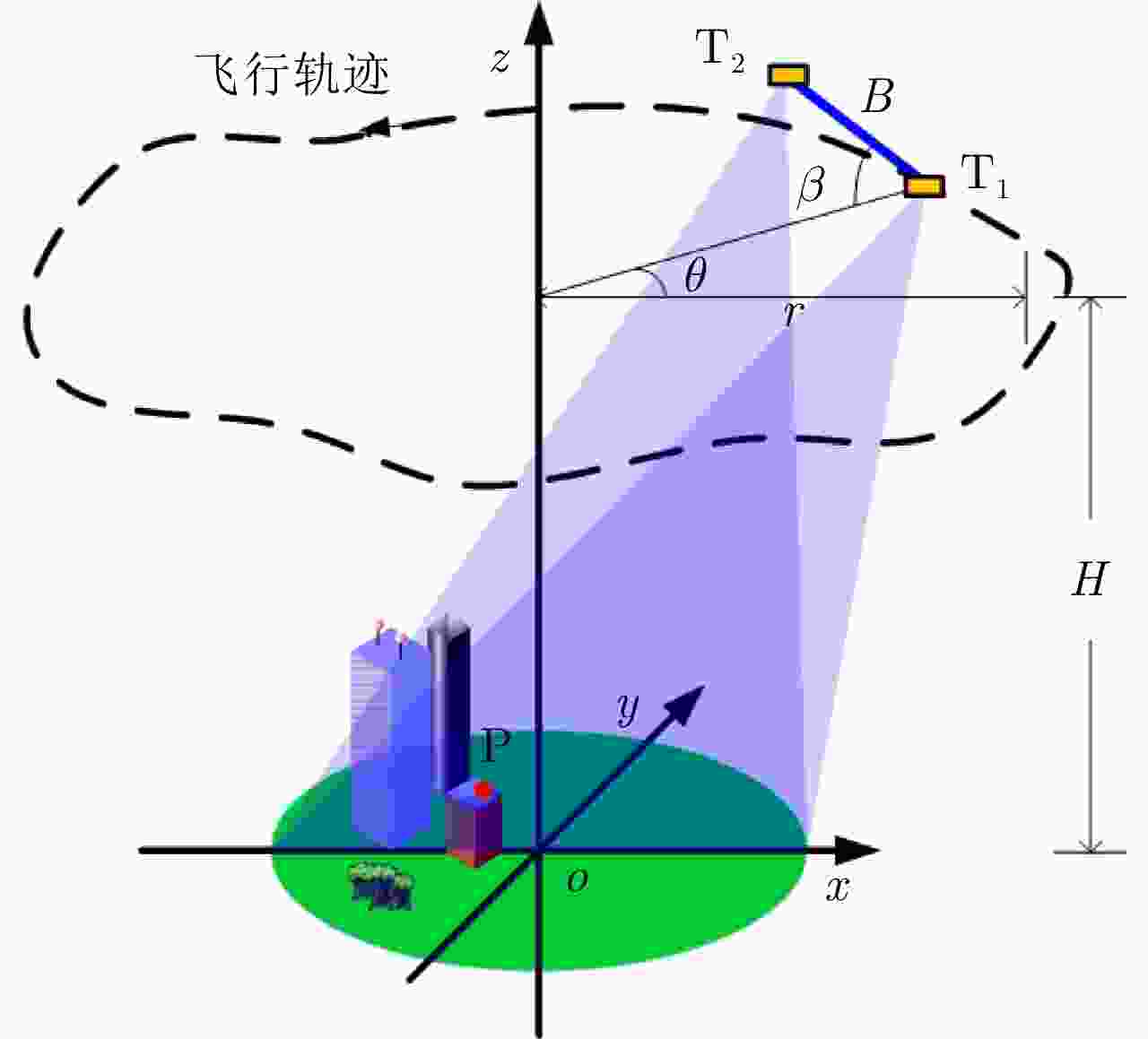
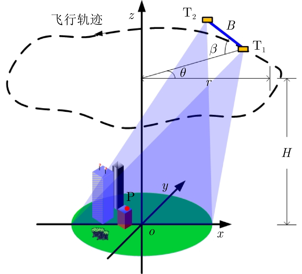
图 1 干涉圆迹SAR观测几何

Figure 1. InCSAR imaging geometry

下载: 全尺寸图片幻灯片

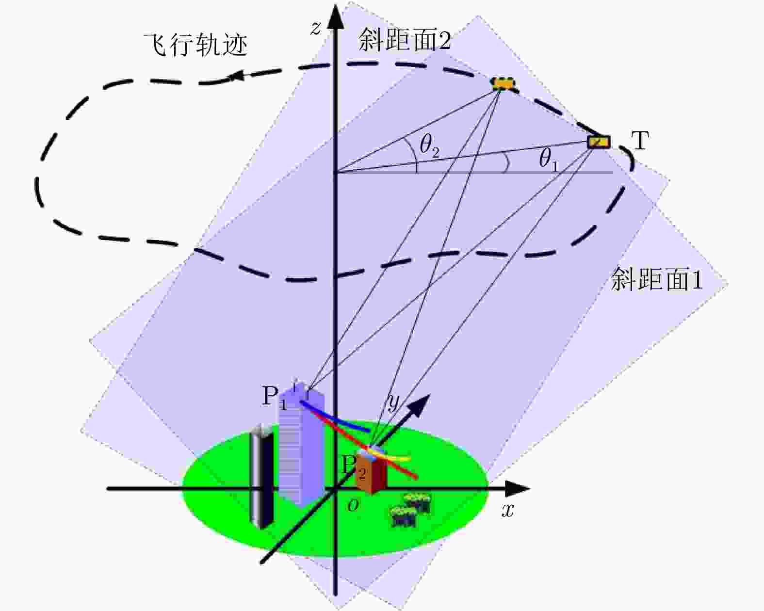
图 2 圆迹SAR解叠掩能力示意图

Figure 2. Layover resolving capability of circular SAR

下载: 全尺寸图片幻灯片

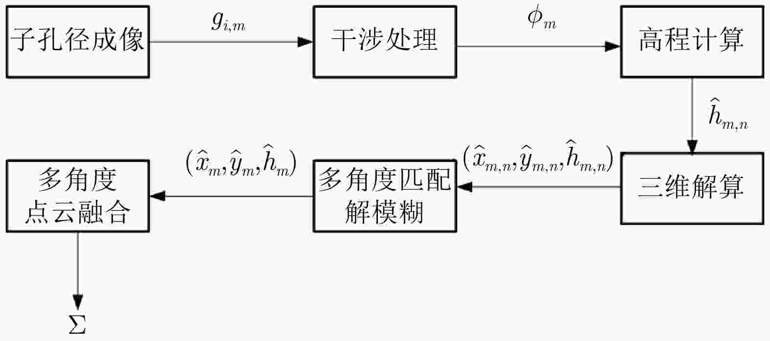
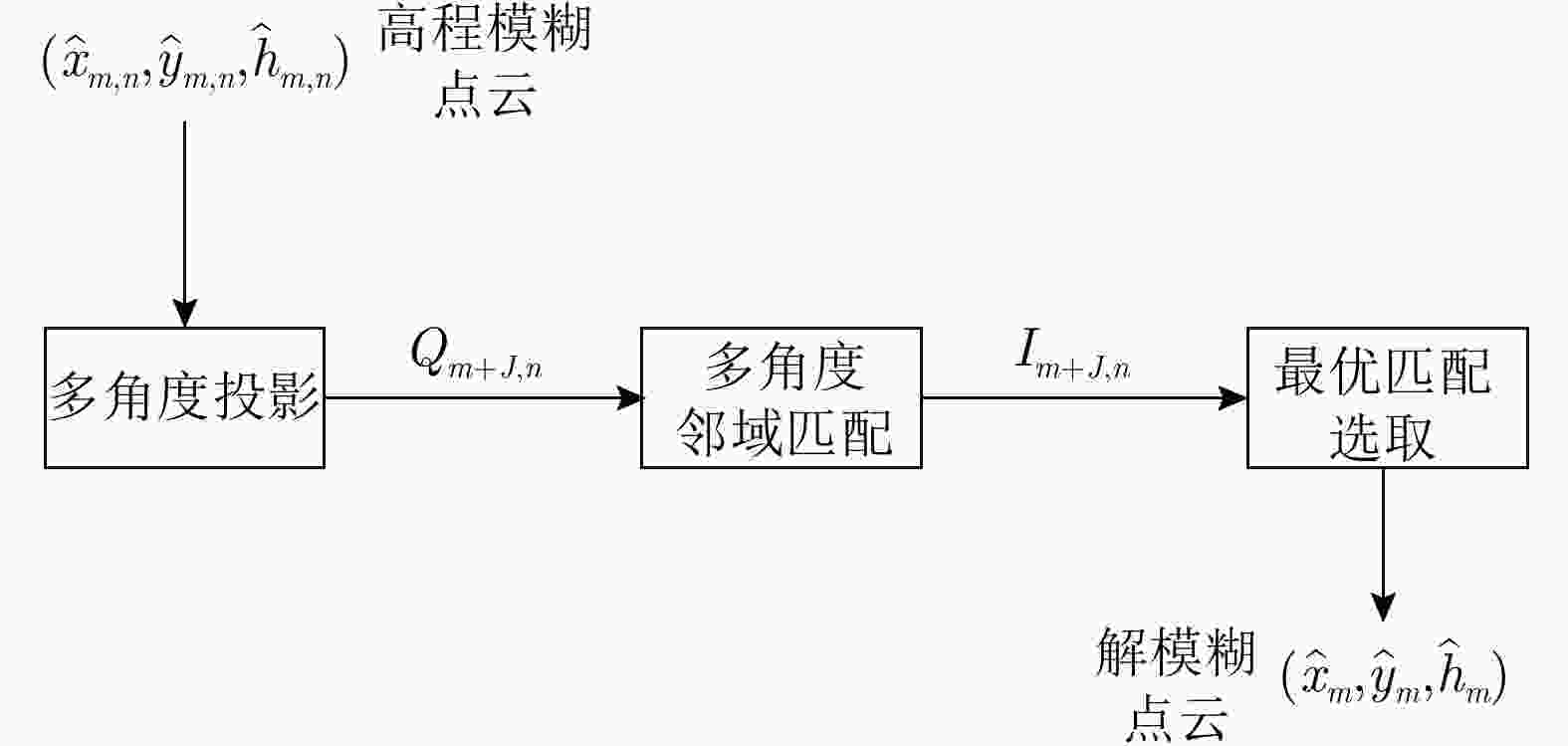
图 3 无先验模型SAR全方位三维成像方法流程图

Figure 3. Flow chart of full-aspect 3D SAR imaging method without prior model

下载: 全尺寸图片幻灯片

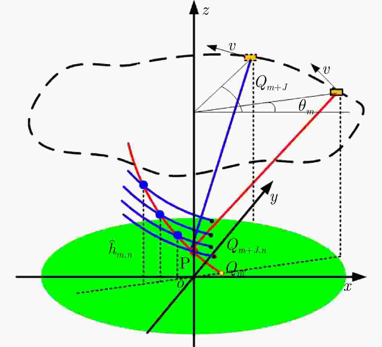
图 4 干涉圆迹SAR瞬时观测几何

Figure 4. Instantaneous geometry of InCAR

下载: 全尺寸图片幻灯片

图 5 多角度解模糊示意图

Figure 5. Diagram of multi-aspect ambiguity resolving

下载: 全尺寸图片幻灯片

图 6 多角度匹配解模糊流程

Figure 6. Flow chart of multi-aspect ambiguity resolving

下载: 全尺寸图片幻灯片

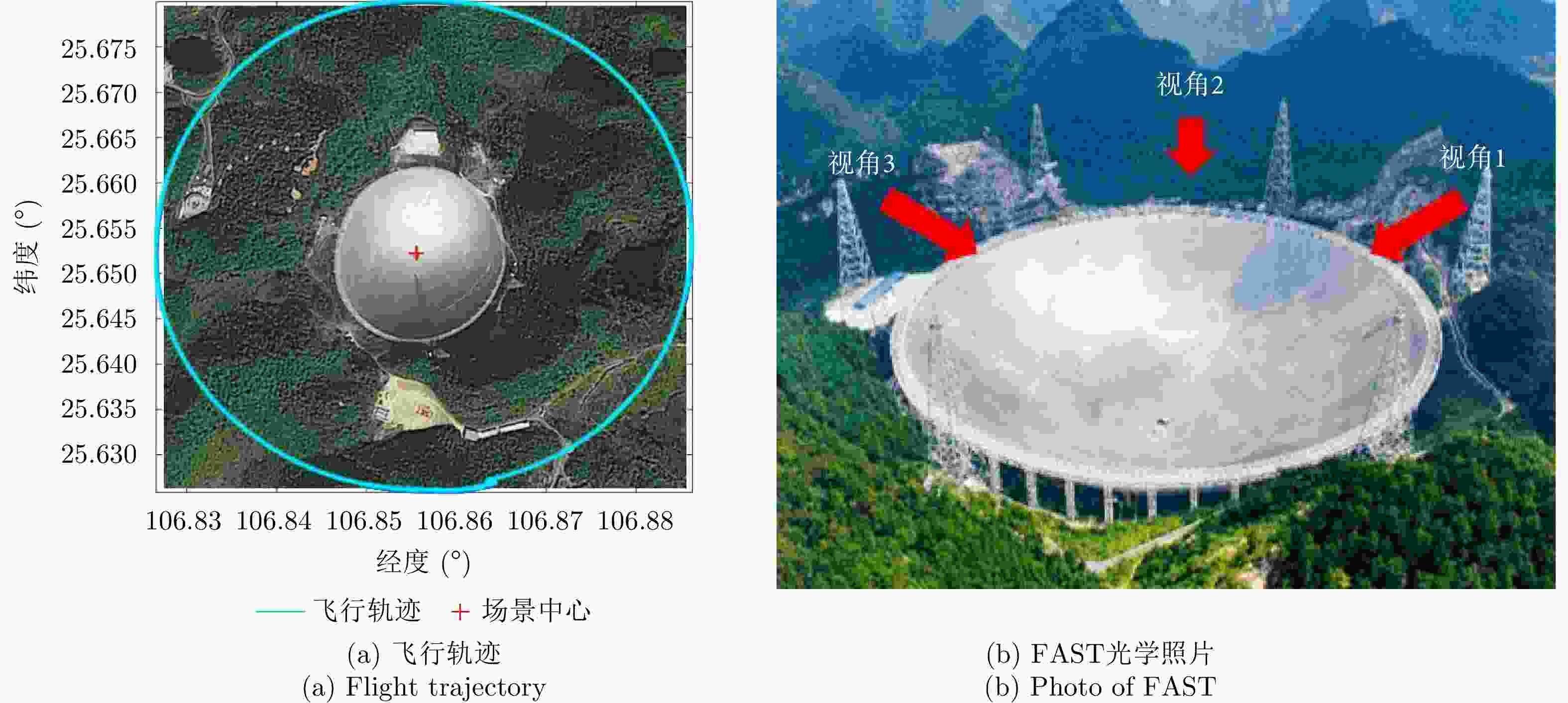
图 7 机载实验飞行轨迹与观测目标

Figure 7. Flight trajectory and the observed object

下载: 全尺寸图片幻灯片

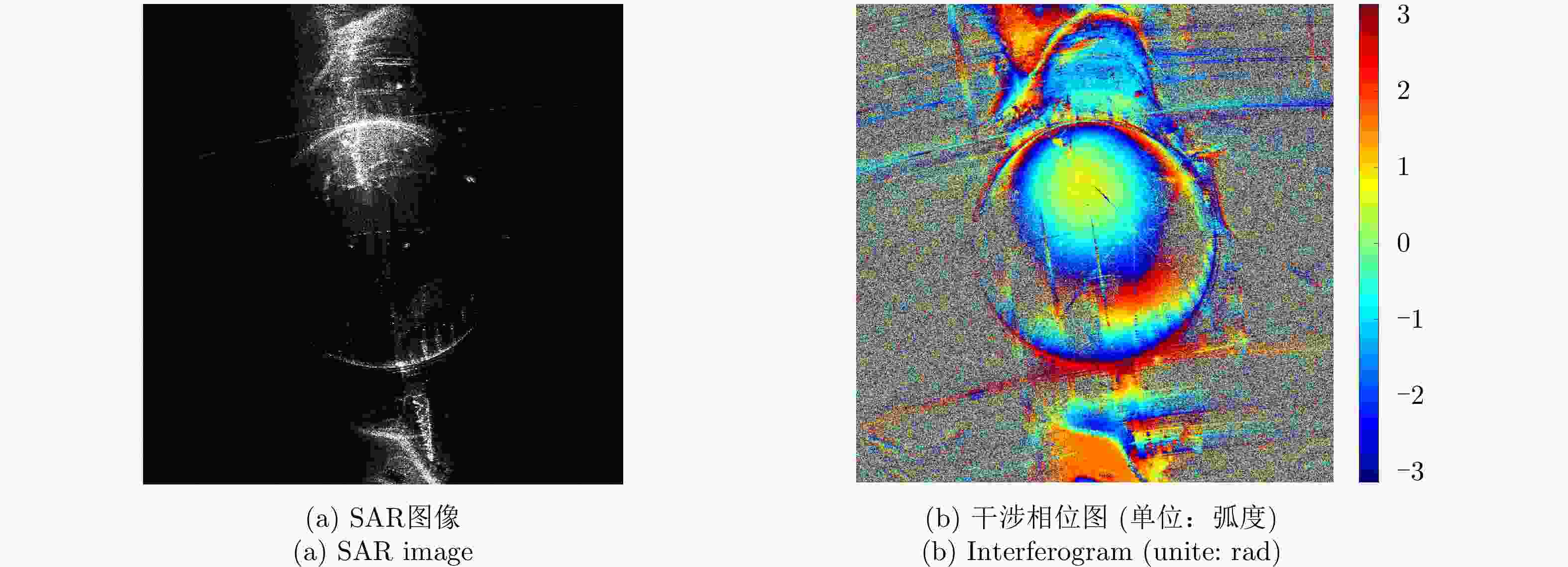
图 8 某子孔径SAR图像与干涉相位图

Figure 8. SAR image and interferogram of certain subapture

下载: 全尺寸图片幻灯片

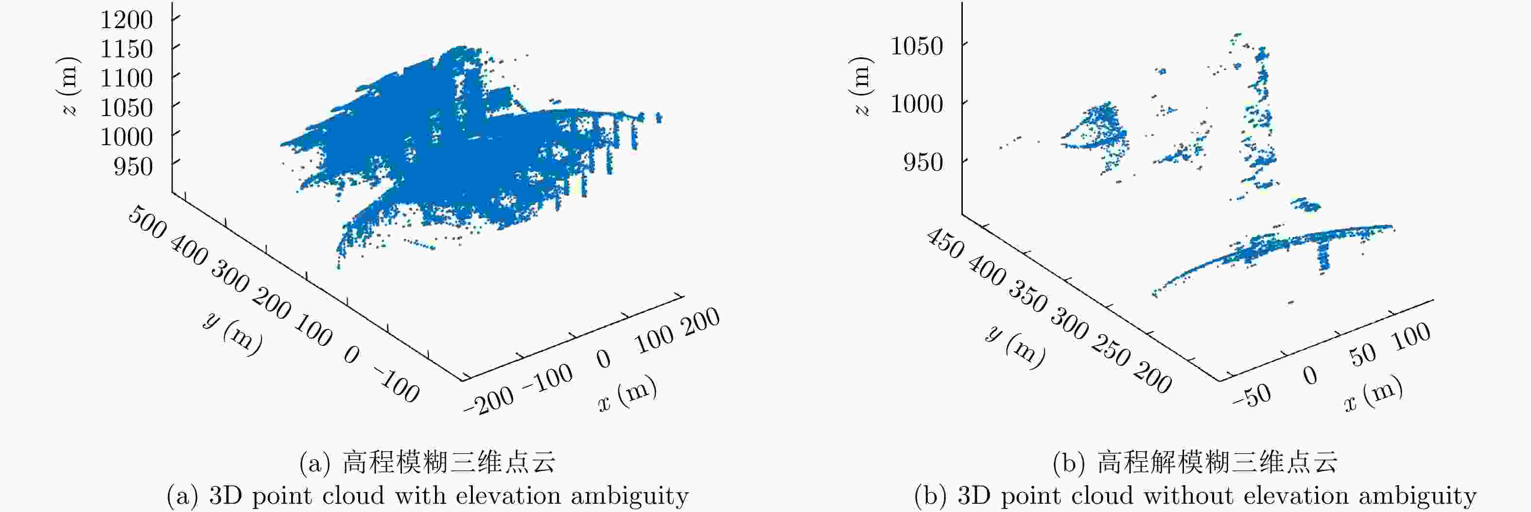
图 9 某子孔径三维点云

Figure 9. 3D point cloud of certain subapture

下载: 全尺寸图片幻灯片

图 10 常规条带SAR图像与全方位三维SAR图像对比

Figure 10. Comparison between conventional stripmap SAR image and full-aspect 3D SAR image

下载: 全尺寸图片幻灯片

表 1 Ka波段机载干涉圆迹SAR实验参数

Table 1. Parameters of Ka-band airborne InCSAR experiment

参数数值参数数值

中心频率 35 GHz 带宽 900 MHz
基线长度 0.156 m 基线倾角 45°
飞行高度 4000 m 飞行半径 3000 m
场景海拔 940 m

下载: 导出CSV

参考文献(39)

[1]	洪文. 圆迹SAR成像技术研究进展[J]. 雷达学报, 2012, 1(2): 124–135. doi: 10.3724/SP.J.1300.2012.20046 HONG Wen. Progress in circular SAR imaging technique[J]. Journal of Radars, 2012, 1(2): 124–135. doi: 10.3724/SP.J.1300.2012.20046
[2]	LIN Yun, HONG Wen, TAN Weixian, et al. Airborne circular SAR imaging: Results at P-band[C]. 2012 IEEE International Geoscience and Remote Sensing Symposium, Munich, Germany, 2012: 5594–5597.
[3]	安道祥, 陈乐平, 冯东, 等. 机载圆周SAR成像技术研究[J]. 雷达学报, 2020, 9(2): 221–242. doi: 10.12000/JR20026 AN Daoxiang, CHEN Leping, FENG Dong, et al. Study of the airborne circular synthetic aperture radar imaging technology[J]. Journal of Radars, 2020, 9(2): 221–242. doi: 10.12000/JR20026
[4]	朱岱寅, 张营, 俞翔, 等. 微型合成孔径雷达成像信号处理技术[J]. 雷达学报, 2019, 8(6): 793–803. doi: 10.12000/JR19094 ZHU Daiyin, ZHANG Ying, YU Xiang, et al. Imaging signal processing technology for miniature synthetic aperture radar[J]. Journal of Radars, 2019, 8(6): 793–803. doi: 10.12000/JR19094
[5]	洪文, 王彦平, 林赟, 等. 新体制SAR三维成像技术研究进展[J]. 雷达学报, 2018, 7(6): 633–654. doi: 10.12000/JR18109 HONG Wen, WANG Yanping, LIN Yun, et al. Research progress on three-dimensional SAR imaging techniques[J]. Journal of Radars, 2018, 7(6): 633–654. doi: 10.12000/JR18109
[6]	LIN Yun, HONG Wen, LI Yang, et al. Study on fine feature description of multi-aspect SAR observations[C]. 2016 IEEE International Geoscience and Remote Sensing Symposium, Beijing, China, 2016: 5682–5685.
[7]	毕辉, 金双, 王潇, 等. 基于高分三号SAR数据的城市建筑高分辨率高维成像[J]. 雷达学报, 2022, 11(1): 40–51. doi: 10.12000/JR21113 BI Hui, JIN Shuang, WANG Xiao, et al. High-resolution high-dimensional imaging of urban building based on GaoFen-3 SAR data[J]. Journal of Radars, 2022, 11(1): 40–51. doi: 10.12000/JR21113
[8]	赵曜, 许俊聪, 全相印, 等. 基于稀疏和低秩结构的层析SAR成像方法[J]. 雷达学报, 2022, 11(1): 52–61. doi: 10.12000/JR21210 ZHAO Yao, XU Juncong, QUAN Xiangyin, et al. Tomographic SAR imaging method based on sparse and low-rank structures[J]. Journal of Radars, 2022, 11(1): 52–61. doi: 10.12000/JR21210
[9]	ERTIN E, AUSTIN C D, SHARMA S, et al. GOTCHA experience report: Three-dimensional SAR imaging with complete circular apertures[C]. SPIE 6568, Algorithms for Synthetic Aperture Radar Imagery XIV, Orlando, United States, 2007: 9–20.
[10]	BAO Qian, LIN Yun, HONG Wen, et al. Holographic SAR tomography image reconstruction by combination of adaptive imaging and sparse Bayesian inference[J]. IEEE Geoscience and Remote Sensing Letters, 2017, 14(8): 1248–1252. doi: 10.1109/LGRS.2017.2704601
[11]	DONG Feng, AN Daoxiang, CHEN Leping, et al. Holographic SAR tomography 3-D reconstruction based on iterative adaptive approach and generalized likelihood ratio test[J]. IEEE Transactions on Geoscience and Remote Sensing, 2021, 59(1): 305–315. doi: 10.1109/TGRS.2020.2994201
[12]	AUSTIN C D, ERTIN E, and MOSES R L. Sparse signal methods for 3-D radar imaging[J]. IEEE Journal of Selected Topics in Signal Processing, 2011, 5(3): 408–423. doi: 10.1109/JSTSP.2010.2090128
[13]	ERTIN E, MOSES R L, and POTTER L C. Interferometric methods for three-dimensional target reconstruction with multipass circular SAR[J]. IET Radar, Sonar & Navigation, 2010, 4(3): 464–473. doi: 10.1049/iet-rsn.2009.0048
[14]	PONCE O, PRATS-IRAOLA P, SCHEIBER R, et al. First airborne demonstration of holographic SAR tomography with fully polarimetric multicircular acquisitions at L-band[J]. IEEE Transactions on Geoscience and Remote Sensing, 2016, 54(10): 6170–6196. doi: 10.1109/TGRS.2016.2582959
[15]	PONCE O, PRATS P, SCHEIBER R, et al. Polarimetric 3-D imaging with airborne holographic SAR tomography over glaciers[C]. 2015 IEEE International Geoscience and Remote Sensing Symposium, Milan, Italy, 2015: 5280–5283.
[16]	PONCE O, JOERG H, SCHEIBER R, et al. First study on holographic SAR tomography over agricultural crops at C-/X-band[C]. 2016 IEEE International Geoscience and Remote Sensing Symposium, Beijing, China, 2016: 7403–7406.
[17]	仇晓兰, 焦泽坤, 杨振礼, 等. 微波视觉三维SAR关键技术及实验系统初步进展[J]. 雷达学报, 2022, 11(1): 1–19. doi: 10.12000/JR22027 QIU Xiaolan, JIAO Zekun, YANG Zhenli, et al. Key technology and preliminary progress of microwave vision 3D SAR experimental system[J]. Journal of Radars, 2022, 11(1): 1–19. doi: 10.12000/JR22027
[18]	刘燕, 谭维贤, 林赟, 等. 基于圆迹SAR的建筑物轮廓信息提取[J]. 电子与信息学报, 2015, 37(4): 946–952. doi: 10.11999/JEIT140717 LIU Yan, TAN Weixian, LIN Yun, et al. An approach of the outlines extraction of building footprints from the circular SAR data[J]. Journal of Electronics &Information Technology, 2015, 37(4): 946–952. doi: 10.11999/JEIT140717
[19]	YU Lingjuan, LIN Yun, LI Yang, et al. Height profile estimation of power lines based on two-dimensional CSAR imagery[J]. IEEE Geoscience and Remote Sensing Letters, 2016, 13(3): 339–343. doi: 10.1109/LGRS.2015.2512285
[20]	ZHANG Ying, ZHU Daiyin, and KONG Yingying. 3-D structure-from-motion retrieval based on circular videosar sequences[C]. 2019 IEEE International Geoscience and Remote Sensing Symposium, Yokohama, Japan, 2019: 134–137.
[21]	CHEN Leping, AN Daoxiang, HUANG Xiaotao, et al. A 3D reconstruction strategy of vehicle outline based on single-pass single-polarization CSAR data[J]. IEEE Transactions on Image Processing, 2017, 26(11): 5545–5554. doi: 10.1109/TIP.2017.2738566
[22]	ZHOU Chaowei, ZHOU Yejian, SUO Zhiyong, et al. Voxel area sculpturing-based 3D scene reconstruction from single-pass CSAR data[J]. Electronics Letters, 2020, 56(11): 566–567. doi: 10.1049/el.2020.0263
[23]	ZHAO Yue, LIN Yun, HONG Wen, et al. Adaptive imaging of anisotropic target based on circular-SAR[J]. Electronics Letters, 2016, 52(16): 1406–1408. doi: 10.1049/el.2016.1764
[24]	赵月, 林赟, 王彦平, 等. 基于圆迹SAR的目标方位散射特征提取研究[J]. 信号处理, 2017, 33(4): 613–617. doi: 10.16798/j.issn.1003-0530.2017.04.024 ZHAO Yue, LIN Yun, WANG Yanping, et al. Target feature extraction on azimuth angles based on circular SAR[J]. Journal of Signal Processing, 2017, 33(4): 613–617. doi: 10.16798/j.issn.1003-0530.2017.04.024
[25]	TENG Fei, HONG Wen, and LIN Yun. Aspect entropy extraction using circular SAR data and scattering anisotropy analysis[J]. Sensors, 2019, 19(2): 346. doi: 10.3390/s19020346
[26]	TENG Fei, LIN Yun, WANG Yanping, et al. An anisotropic scattering analysis method based on the statistical properties of multi-angular SAR images[J]. Remote Sensing, 2020, 12(13): 2152. doi: 10.3390/rs12132152
[27]	LI Yang, YIN Qiang, LIN Yun, et al. Anisotropy scattering detection from multiaspect signatures of circular polarimetric SAR[J]. IEEE Geoscience and Remote Sensing Letters, 2018, 15(10): 1575–1579. doi: 10.1109/LGRS.2018.2850859
[28]	XUE Feiteng, LIN Yun, HONG Wen, et al. An improved H/α unsupervised classification method for circular PolSAR images[J]. IEEE Access, 2018, 6: 34296–34306. doi: 10.1109/ACCESS.2018.2838329
[29]	XU Feng, LI Yongchen, and JIN Yaqiu. Polarimetric-anisotropic decomposition and anisotropic entropies of high-resolution SAR images[J]. IEEE Transactions on Geoscience and Remote Sensing, 2016, 54(9): 5467–5482. doi: 10.1109/TGRS.2016.2565693
[30]	杨彦辉, 林赟, 洪文. 利用星载SAR单轨多角度地距图像提取高程信息[J]. 测绘科学, 2019, 44(7): 96–104. doi: 10.16251/j.cnki.1009-2307.2019.07.015 YANG Yanhui, LIN Yun, and HONG Wen. Elevation extraction from multi-angle and ground-range images in single orbit based on spaceborne SAR[J]. Science of Surveying and Mapping, 2019, 44(7): 96–104. doi: 10.16251/j.cnki.1009-2307.2019.07.015
[31]	FENG Shanshan, LIN Yun, WANG Yanping, et al. DEM generation with a scale factor using multi-aspect SAR imagery applying radargrammetry[J]. Remote Sensing, 2020, 12(3): 556. doi: 10.3390/rs12030556
[32]	ZHANG Hanqing, LIN Yun, FENG Shanshan, et al. 3-D target reconstruction using C-band circular SAR imagery based on background constraints[C]. 2021 IEEE International Geoscience and Remote Sensing Symposium, Brussels, Belgium, 2021: 2923–2926.
[33]	FENG Shanshan, LIN Yun, WANG Yanping, et al. 3D point cloud reconstruction using inversely mapping and voting from single pass CSAR images[J]. Remote Sensing, 2021, 13(17): 3534. doi: 10.3390/rs13173534
[34]	LIN Yun, HONG Wen, TAN Weixian, et al. Interferometric circular SAR method for three-dimensional imaging[J]. IEEE Geoscience and Remote Sensing Letters, 2011, 8(6): 1026–1030. doi: 10.1109/LGRS.2011.2150732
[35]	LIN Yun, BAO Qian, HOU Liying, et al. Full-aspect 3D target reconstruction of interferometric circular SAR[C]. SPIE 10004, Image and Signal Processing for Remote Sensing XXII, Edinburgh, UK, 2016: 424–432.
[36]	侯丽英, 林赟, 洪文. 干涉圆迹SAR的目标三维重建方法研究[J]. 雷达学报, 2016, 5(5): 538–547. doi: 10.12000/JR16009 HOU Liying, LIN Yun, and HONG Wen. Three-dimensional reconstruction method study based on interferometric circular SAR[J]. Journal of Radars, 2016, 5(5): 538–547. doi: 10.12000/JR16009
[37]	刘燕, 林赟, 谭维贤, 等. 基于圆迹干涉SAR的DEM提取[J]. 电子与信息学报, 2015, 37(6): 1463–1469. doi: 10.11999/JEIT141022 LIU Yan, LIN Yun, TAN Weixian, et al. DEM extraction based on interferometric circular SAR[J]. Journal of Electronics &Information Technology, 2015, 37(6): 1463–1469. doi: 10.11999/JEIT141022
[38]	LIU Jiayin, QIU Xiaolan, and HONG Wen. Automated ortho-rectified SAR image of GF-3 satellite using reverse-range-Doppler method[C]. 2016 IEEE International Geoscience and Remote Sensing Symposium, Beijing, China, 2016: 4445–4448.
[39]	YOO J C and HAN T H. Fast normalized cross-correlation[J]. Circuits, Systems and Signal Processing, 2009, 28(6): 819–843. doi: 10.1007/s00034-009-9130-7

施引文献

期刊类型引用(4)

1.	葛津津，周浩，凌天庆. 一种应用于脉冲探地雷达前端的探测子系统. 电子测量技术. 2022(04): 27-32 . 百度学术
2.	尹诗，郭伟. 用于探地雷达的超宽带天线设计与仿真. 电子设计工程. 2018(03): 98-102 . 百度学术
3.	宋立伟，张超，洪涛. 冲击波载荷对平面阵列天线电性能的影响. 电子机械工程. 2017(04): 1-5+58 . 百度学术
4.	尹德，叶盛波，刘晋伟，纪奕才，刘小军，方广有. 一种用于高速公路探地雷达的新型时域超宽带TEM喇叭天线. 雷达学报. 2017(06): 611-618 . 本站查看

其他类型引用(6)

资源附件(0)

访问统计

图(10) / 表(1)

计量

文章访问数: 1290
HTML全文浏览量: 647
PDF下载量: 231
被引次数: 10

1. Introduction
2. Conformal FDA-MIMO Radar
2.1 General conformal FDA-MIMO signal model
2.2 CRLB of conformal FDA-MIMO
3. Reduced-Dimension Target Parameter Estimation Algorithm
4. Simulation Results
4.1 Analysis of computational complexity
4.2 Single target parameter estimation
4.3 Multiple targets parameter estimation
5. Conclusion

1. Introduction
2. Conformal FDA-MIMO Radar
2.1 General conformal FDA-MIMO signal model
2.2 CRLB of conformal FDA-MIMO
3. Reduced-Dimension Target Parameter Estimation Algorithm
4. Simulation Results
4.1 Analysis of computational complexity
4.2 Single target parameter estimation
4.3 Multiple targets parameter estimation
5. Conclusion

参考文献(39)

施引文献

资源附件(0)

访问统计

无先验模型复杂结构设施SAR全方位三维成像方法研究

DOI: 10.12000/JR22148

通讯作者:
洪文 whong@mail.ie.ac.cn

计量

Research on Full-aspect Three-dimensional SAR Imaging Method for Complex Structural Facilities without Prior Model

Corresponding author: HONG Wen, whong@mail.ie.ac.cn

1. Introduction

2. Conformal FDA-MIMO Radar

2.1 General conformal FDA-MIMO signal model

2.2 CRLB of conformal FDA-MIMO

3. Reduced-Dimension Target Parameter Estimation Algorithm

4. Simulation Results

4.1 Analysis of computational complexity

4.2 Single target parameter estimation

4.3 Multiple targets parameter estimation

5. Conclusion

期刊类型引用(4)

其他类型引用(6)

计量

目录

1. Introduction

2. Conformal FDA-MIMO Radar

2.1 General conformal FDA-MIMO signal model

2.2 CRLB of conformal FDA-MIMO

3. Reduced-Dimension Target Parameter Estimation Algorithm

4. Simulation Results

4.1 Analysis of computational complexity

4.2 Single target parameter estimation

4.3 Multiple targets parameter estimation

5. Conclusion

期刊介绍

联系我们

参数	数值	参数	数值
中心频率	35 GHz	带宽	900 MHz
基线长度	0.156 m	基线倾角	45°
飞行高度	4000 m	飞行半径	3000 m
场景海拔	940 m

无先验模型复杂结构设施SAR全方位三维成像方法研究

DOI: 10.12000/JR22148

通讯作者: 洪文 whong@mail.ie.ac.cn

计量

出版历程

Research on Full-aspect Three-dimensional SAR Imaging Method for Complex Structural Facilities without Prior Model

Corresponding author: HONG Wen, whong@mail.ie.ac.cn

1. Introduction

2. Conformal FDA-MIMO Radar

2.1 General conformal FDA-MIMO signal model

2.2 CRLB of conformal FDA-MIMO

3. Reduced-Dimension Target Parameter Estimation Algorithm

4. Simulation Results

4.1 Analysis of computational complexity

4.2 Single target parameter estimation

4.3 Multiple targets parameter estimation

5. Conclusion

期刊类型引用(4)

其他类型引用(6)

计量

出版历程

目录

1. Introduction

2. Conformal FDA-MIMO Radar

2.1 General conformal FDA-MIMO signal model

2.2 CRLB of conformal FDA-MIMO

3. Reduced-Dimension Target Parameter Estimation Algorithm

4. Simulation Results

4.1 Analysis of computational complexity

4.2 Single target parameter estimation

4.3 Multiple targets parameter estimation

5. Conclusion

期刊介绍

联系我们

通讯作者:
洪文 whong@mail.ie.ac.cn