基于自学习稀疏先验的三维SAR成像方法

王谋; 韦顺军; 沈蓉; 周梓晨; 师君; 张晓玲

doi:10.12000/JR22101

基于自学习稀疏先验的三维SAR成像方法

DOI: 10.12000/JR22101

电子科技大学信息与通信工程学院成都 611731

基金项目: 国家自然科学基金(61671113, 61501098)，国家重点研发计划项目(2017-YFB0502700)，国家留学基金(202106070063)，高分对地观测青年基金(GFZX04061502)

详细信息

作者简介:
王　谋，博士生，主要研究方向为雷达信号处理、压缩感知、机器学习等

韦顺军，博士，副教授，主要研究方向为雷达信号处理、压缩感知、SAR成像系统、SAR图像智能解译等

沈　蓉，硕士生，主要研究方向为三维SAR成像

周梓晨，硕士生，主要研究方向为三维SAR成像、雷达信号处理

师　君，博士，副教授，主要研究方向为雷达信号处理、SAR成像系统、SAR图像智能解译等

张晓玲，博士，教授，主要研究方向为雷达信号处理、SAR成像系统、SAR图像智能解译等

通讯作者:
韦顺军 weishunjun@uestc.edu.cn

责任主编：仇晓兰 Corresponding Editor: QIU Xiaolan
中图分类号: TN957.52
计量
- 文章访问数:
- HTML全文浏览量:
- PDF下载量:
- 被引次数: 0
出版历程
- 收稿日期: 2022-05-24
- 修回日期: 2022-07-09
- 网络出版日期: 2022-07-25
- 刊出日期: 2023-02-28

3D SAR Imaging Method Based on Learned Sparse Prior（in English）

School of Information and Communication Engineering, University of Electronic Science and Technology of China, Chengdu 611731, China

Funds: The National Natural Science Foundation of China (61671113, 61501098), The National Key Research and Development Program of China (2017-YFB0502700), The China Scholarship Council (202106070063), The High-Resolution Earth Observation Youth Foundation (GFZX04061502)

More Information

Corresponding author: WEI Shunjun, weishunjun@uestc.edu.cn

摘要

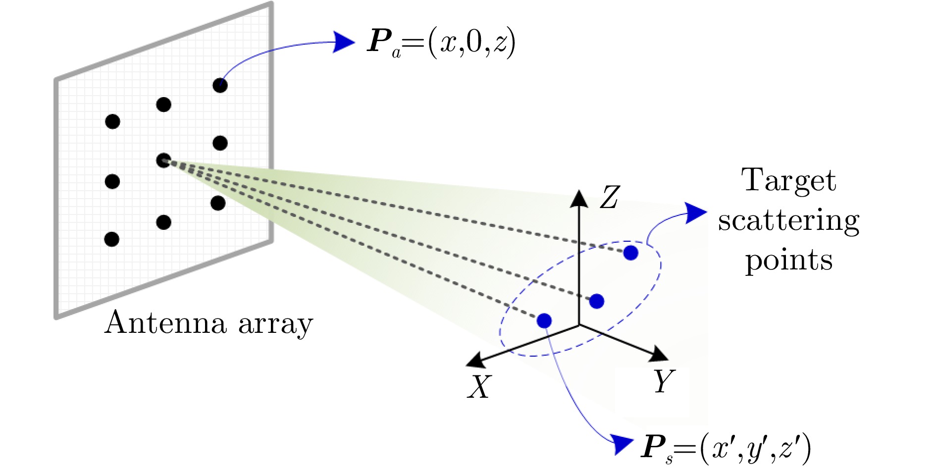
摘要: 合成孔径雷达三维成像技术(3D SAR)能通过孔径维度扩展实现三维成像能力，但数据维度大、系统实现难、成像分辨率低。压缩感知稀疏重构技术在简化3D SAR系统、提升成像质量等方面展现出巨大潜力，但面临计算复杂度高、参数设置困难、弱稀疏场景适应差等新问题，制约了其实际应用。针对上述问题，该文结合卷积神经网络的特征学习及迭代算法的深度展开理论，提出了基于自学习稀疏先验的3D SAR成像方法。首先，探讨了常规3D SAR稀疏成像中矩阵向量线性表征模型的局限性，引入成像算子提升成像算法处理效率。其次，讨论了迭代算法映射网络的深度展开模型和实现方式，包括网络拓扑结构设计、算法参数的优化约束及网络的训练方法。最后，通过仿真数据和地面实验，证明了所提方法在提升成像精度的同时，其运行时间较传统稀疏成像算法降低一个数量级。
- 三维SAR /
- 深度学习 /
- 深度展开 /
- 稀疏表征 /
- 稀疏成像
Abstract: The development of 3D Synthetic Aperture Radar (SAR) imaging is currently hampered by issues such as high data dimension, high system complexity, and low imaging processing efficiency. Sparse SAR imaging has grown in importance as a research branch in SAR imaging due to the high potential of sparse signal processing techniques based on Compressed Sensing (CS) to show high potential in reducing system complexity and improving imaging quality. However, traditional sparse imaging methods are still constrained by high computational complexity, nontrivial parameter tuning, and poor adaptability to weakly sparse scenes. To address these issues, we propose a new 3D SAR imaging method based on learned sparse priors inspired by the deep unfolding concept. First, the limitations of the matrix-vector linear representation model are discussed, and an imaging operator is introduced to improve the algorithm’s imaging efficiency. Furthermore, this research focuses on algorithm network details, such as network topology design, the problem of complex-valued propagations, optimization constraints of algorithm parameters, and network training details. Finally, through simulations and measured experiments, it is proved that the proposed method can improve the imaging accuracy while reducing the running time by more than one order of magnitude compared with the conventional sparse imaging algorithms.
- 3D SAR /
- Deep learning /
- Deep unfolding /
- Sparse representation /
- Sparse imaging

HTML全文

图 1 三维SAR成像几何模型

Figure 1. 3D SAR imaging geometry

下载: 全尺寸图片幻灯片

图 2 所提LSISTA网络结构示意图

Figure 2. The structure of the proposed LSISTA

下载: 全尺寸图片幻灯片

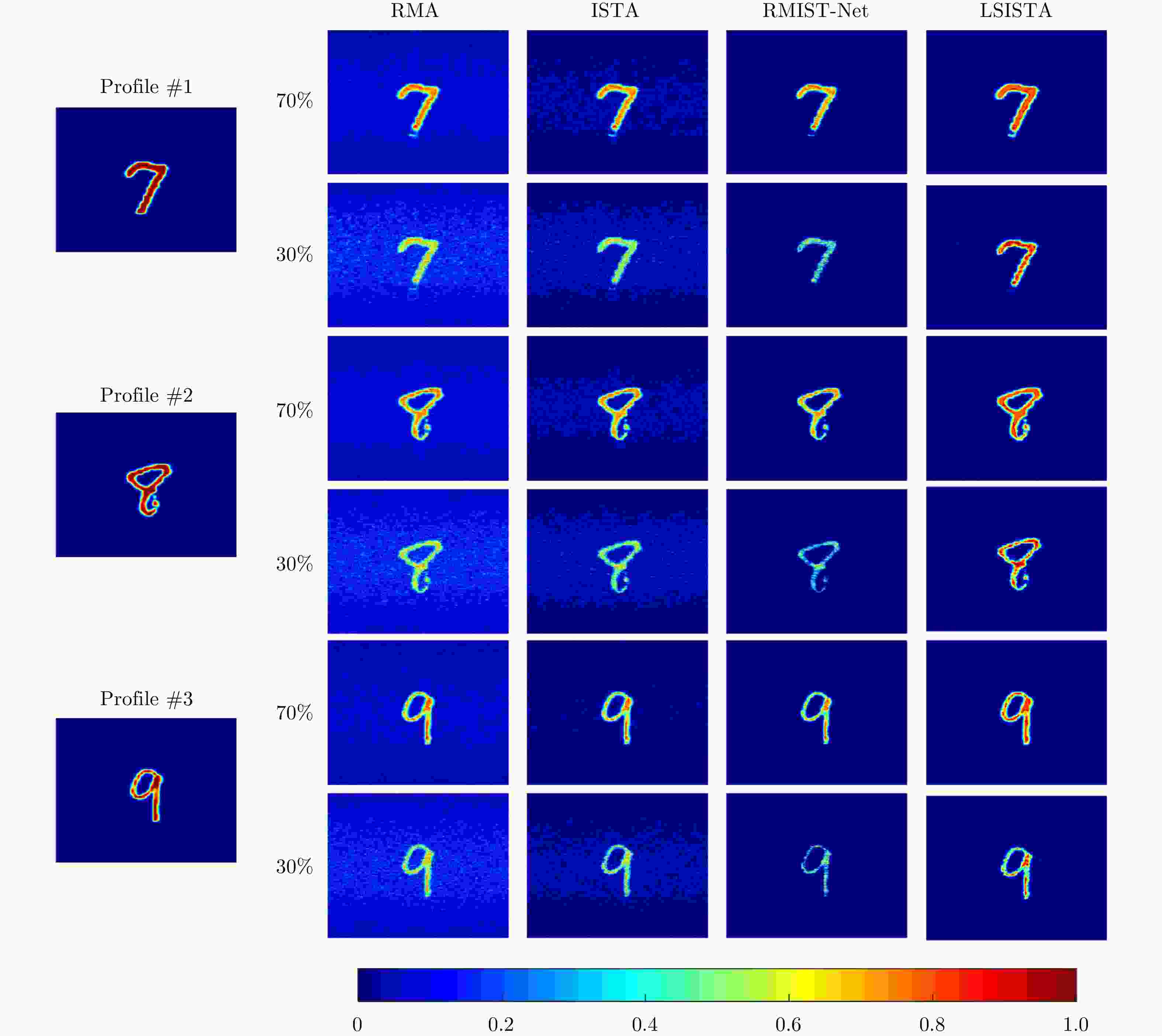
图 3 各算法在采样率分别为70%和30%时的重构结果

Figure 3. Reconstructions of different algorithms in cases of sampling rate being 70% and 30%, respectively

下载: 全尺寸图片幻灯片

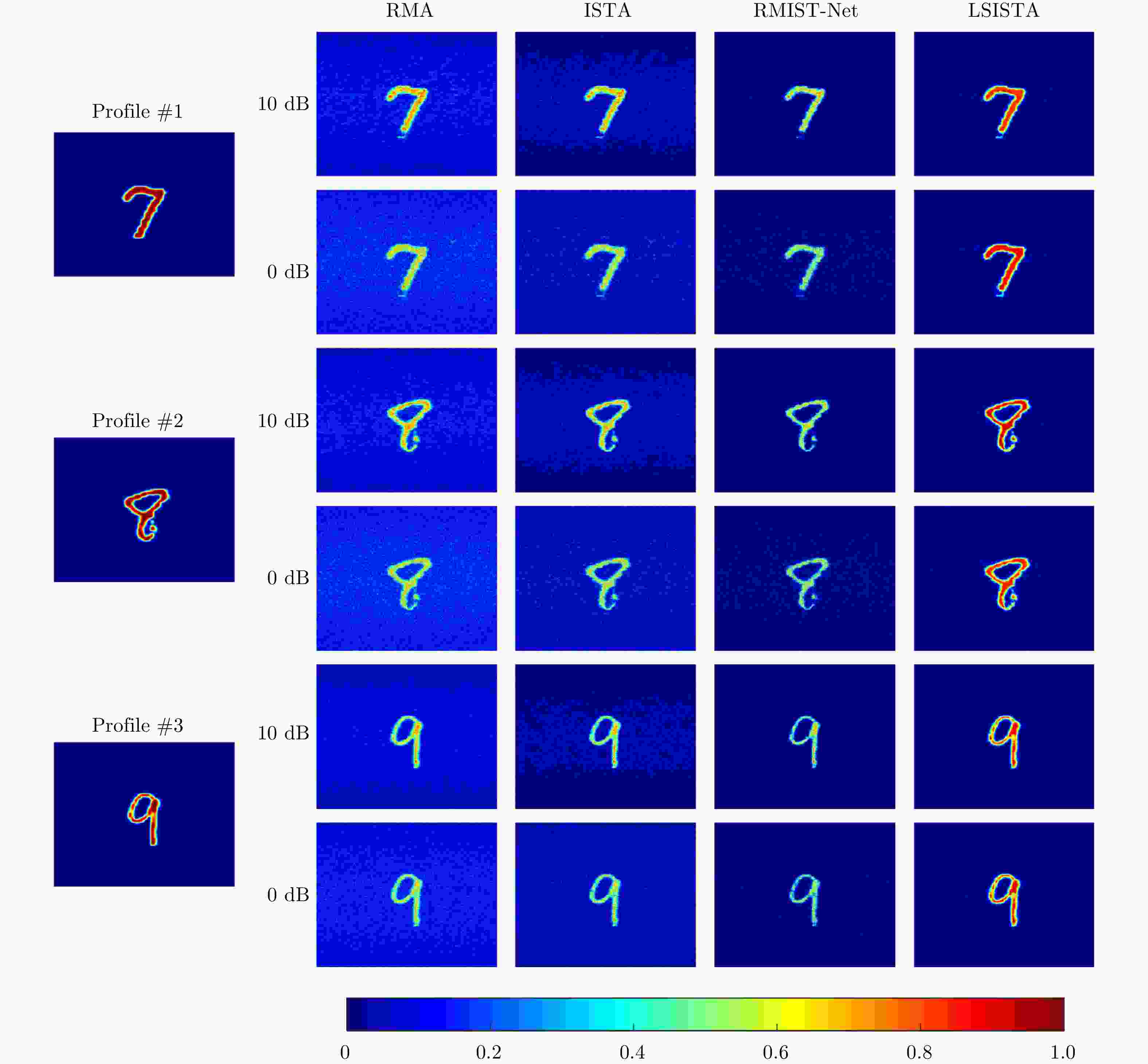
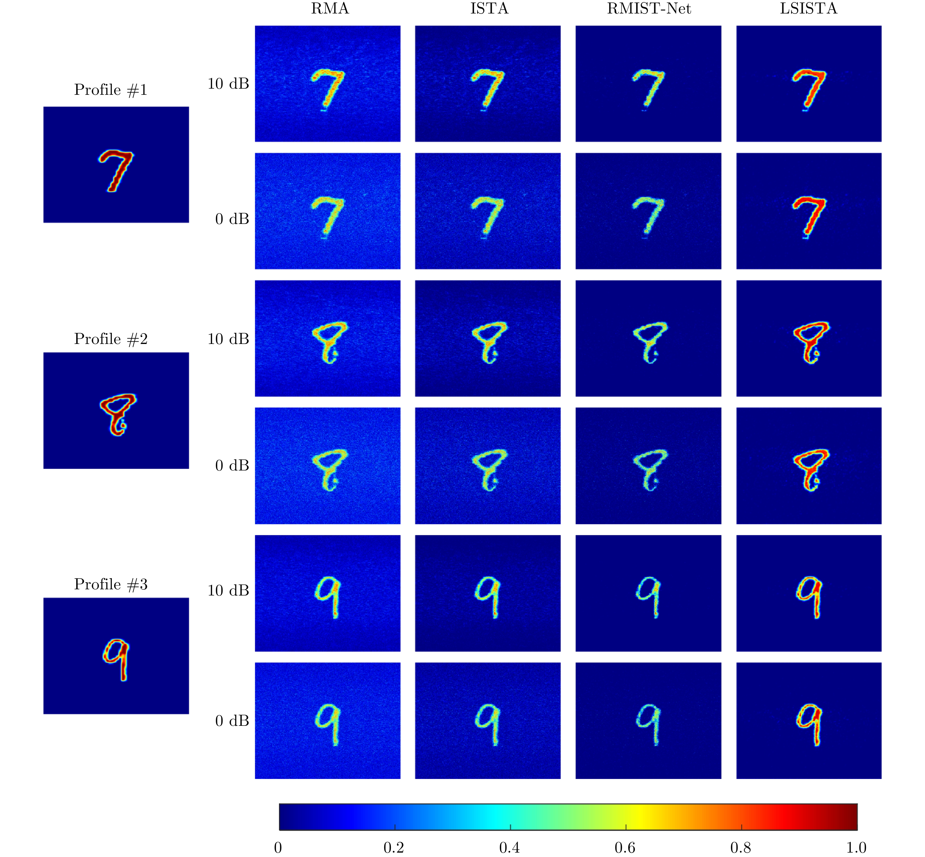
图 4 各算法在SNR分别为10 dB和0 dB时的重构结果

Figure 4. Reconstructions of different algorithms in cases of SNR being 10 dB and 0 dB, respectively

下载: 全尺寸图片幻灯片

图 5 F16三维模型

Figure 5. 3D F16 model

下载: 全尺寸图片幻灯片

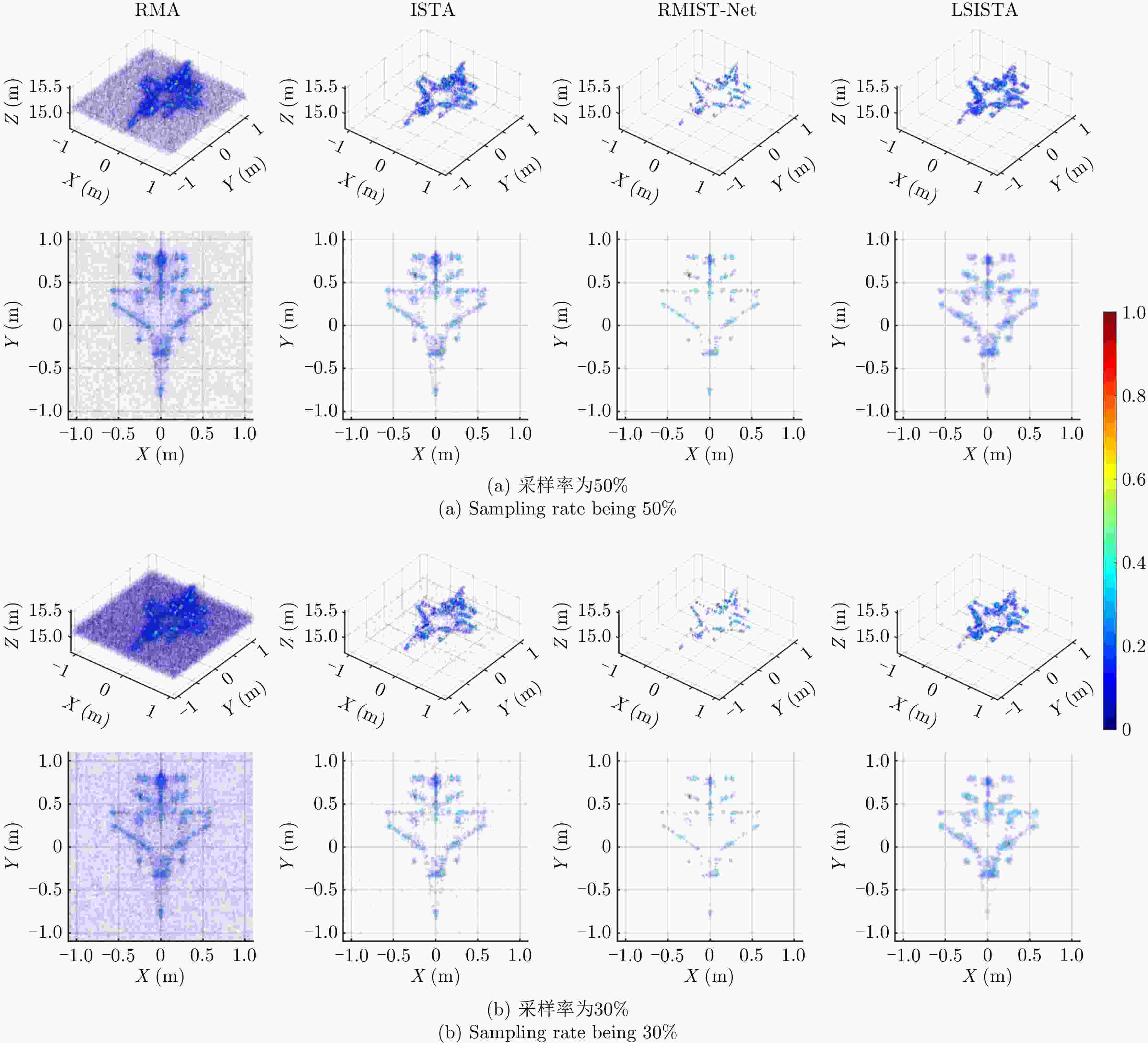
图 6 各算法在采样率为50%和30%时的三维仿真成像结果

Figure 6. 3D imaging results of different algorithms in cases of sampling rate being 50% and 30%

下载: 全尺寸图片幻灯片

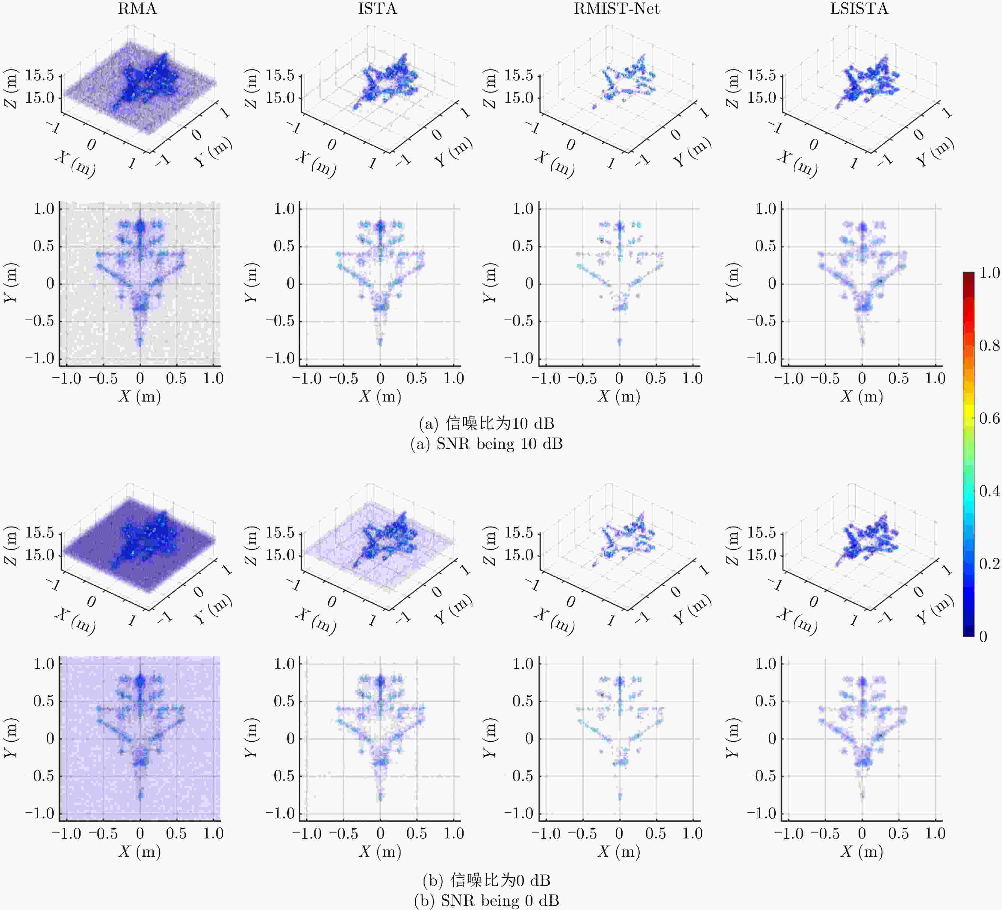
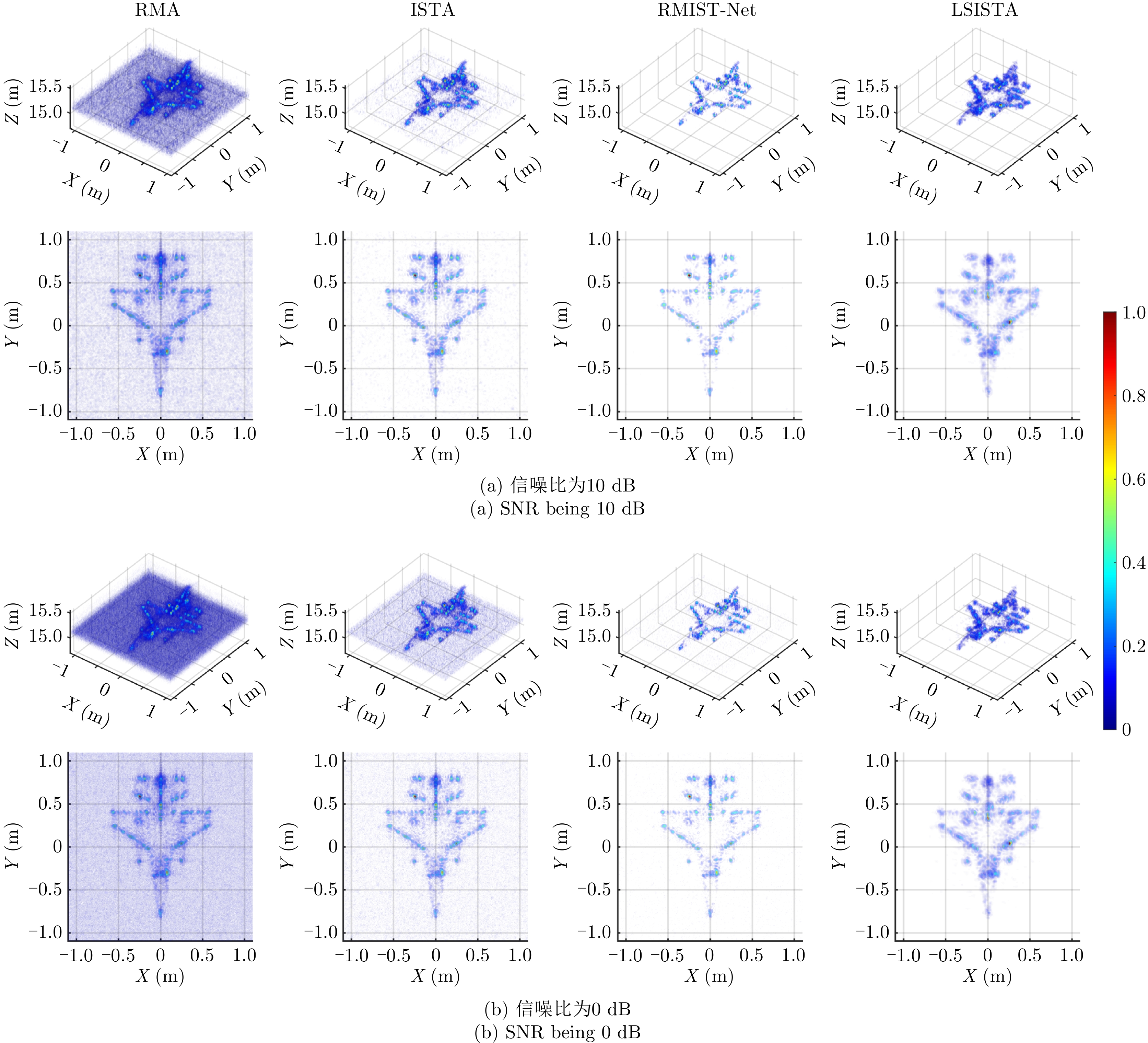
图 7 各算法在信噪比分别为10 dB和0 dB时的三维仿真成像结果

Figure 7. 3D imaging results of different algorithms in cases of SNR being 10 dB and 0 dB

下载: 全尺寸图片幻灯片

图 8 毫米波三维SAR验证平台及实验场景

Figure 8. 3D mmW SAR imaging system and experimental scenarios

下载: 全尺寸图片幻灯片

图 9 各算法在采样率为50%和30%时钢片测试板的三维成像结果

Figure 9. 3D imaging results of the testing steel chip by different algorithms when sampling rate are 50% and 30%

下载: 全尺寸图片幻灯片

图 10 各算法在采样率为50%和30%时隐匿刀具的成像结果

Figure 10. Imaging results of conceal knives by different algorithms when sampling rate are 50% and 30%

下载: 全尺寸图片幻灯片

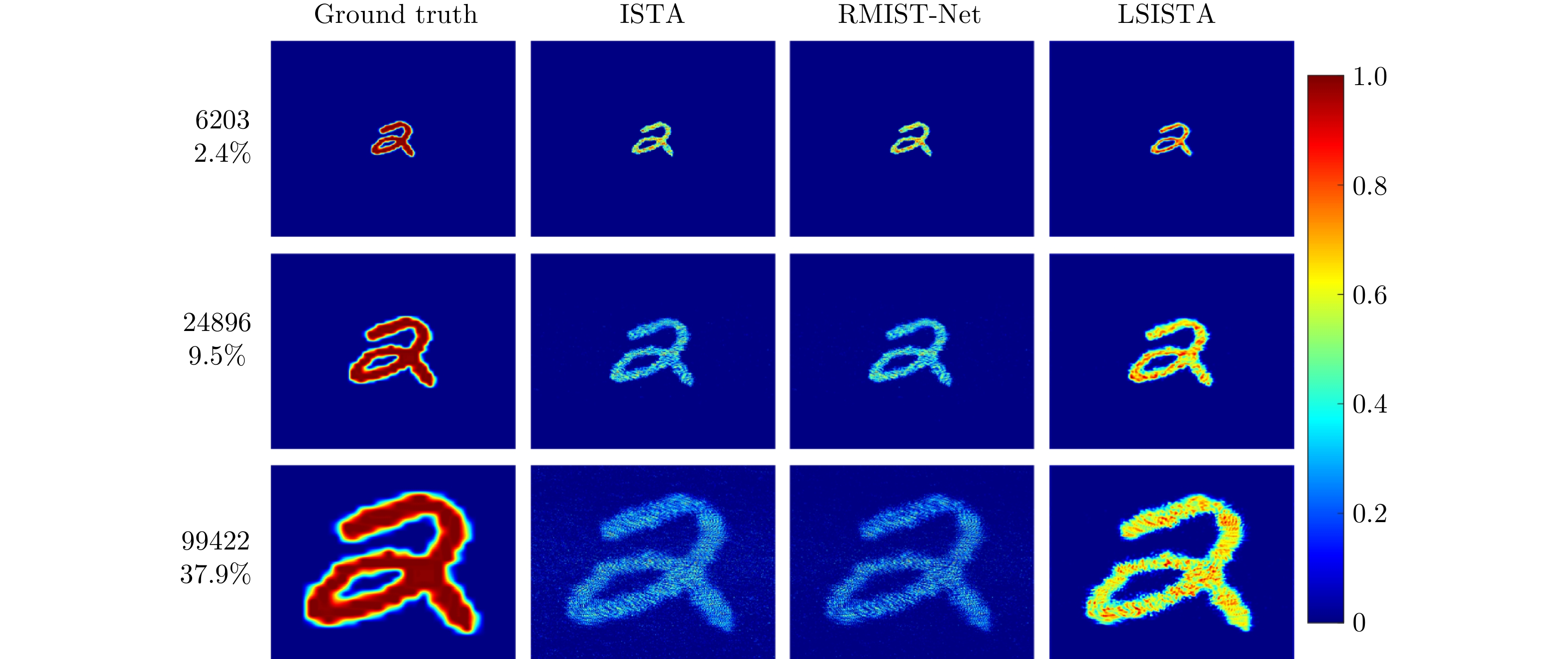
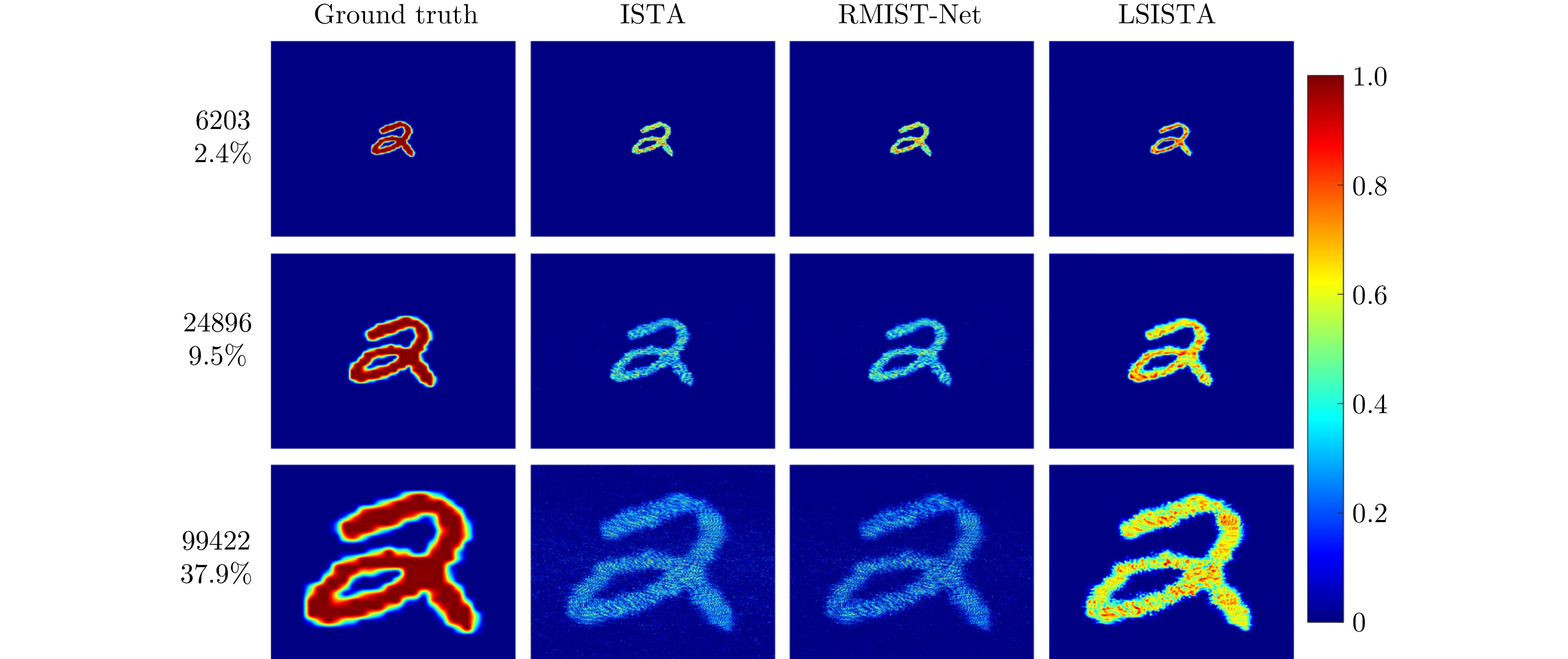
图 11 各稀疏成像算法在不同目标点数时的成像结果

Figure 11. Imaging results of different algorithms in cases of the different number of scatterers

下载: 全尺寸图片幻灯片

图 1 3D SAR imaging geometry

下载: 全尺寸图片幻灯片

图 2 Structure of the proposed LSISTA

下载: 全尺寸图片幻灯片

图 3 Reconstructions of different algorithms in cases of sampling rate being 70% and 30%, respectively

下载: 全尺寸图片幻灯片

图 4 Reconstructions of different algorithms in cases of SNR being 10 and 0 dB, respectively

下载: 全尺寸图片幻灯片

图 5 3D F16 model

下载: 全尺寸图片幻灯片

图 6 Imaging results of different algorithms in cases of sampling rate being 50% and 30%

下载: 全尺寸图片幻灯片

图 7 Imaging results of different algorithms in cases of SNR being 10 and 0 dB

下载: 全尺寸图片幻灯片

图 8 3D mmW SAR imaging system and experimental scenarios

下载: 全尺寸图片幻灯片

图 9 3D Imaging results of the testing steel chip by different algorithms when sampling rates are 50% and 30%

下载: 全尺寸图片幻灯片

图 10 Imaging results of conceal knives by different algorithms when sampling rates are 50% and 30%

下载: 全尺寸图片幻灯片

图 11 Imaging results of different algorithms in cases of different numbers of scatterers

下载: 全尺寸图片幻灯片

算法1 基于核函数的ISTA稀疏成像算法
Alg. 1 ISTA sparse imaging algorithm based on kernel functions
输入：稀疏降采样回波E，相位传播矩阵P，迭代步长$\tau $，迭代　　　　层数T
输出：稀疏成像结果$ {{\boldsymbol{X}}^{\left( T \right)}} $
初始化：$t = 1$, ${{\boldsymbol{X}}^{\left( 0 \right)}} = {\mathcal{M}^{\text{H}}}\left( {{\boldsymbol{E}},{{\bar {\boldsymbol{P}}}}} \right)$；
循环开始
(1) 更新迭代残差：$ {{\boldsymbol{V}}^{\left( t \right)}} = {\boldsymbol{E}} - \mathcal{M}\left( {{{\boldsymbol{X}}^{\left( {t - 1} \right)}},{\boldsymbol{\bar P}}} \right) $；
(2) 梯度下降粗估计：$ {{\boldsymbol{R}}^{\left( t \right)}} = {{\boldsymbol{X}}^{\left( {t - 1} \right)}} + \tau {\mathcal{M}^{\text{H}}}\left( {{{\boldsymbol{V}}^{\left( t \right)}},{\boldsymbol{P}}} \right) $；
(3) 软阈值收缩去噪： ${ {\boldsymbol{X} }^{\left( t \right)} } = {{\rm{soft}}} \left( { { {\boldsymbol{R} }^{\left( t \right)} },\lambda } \right)$, $t = t + 1$；
(4) 迭代判定：若$t \le T$，则重复步骤(1)—步骤(4)；否则，结束循环。
循环结束

下载: 导出CSV

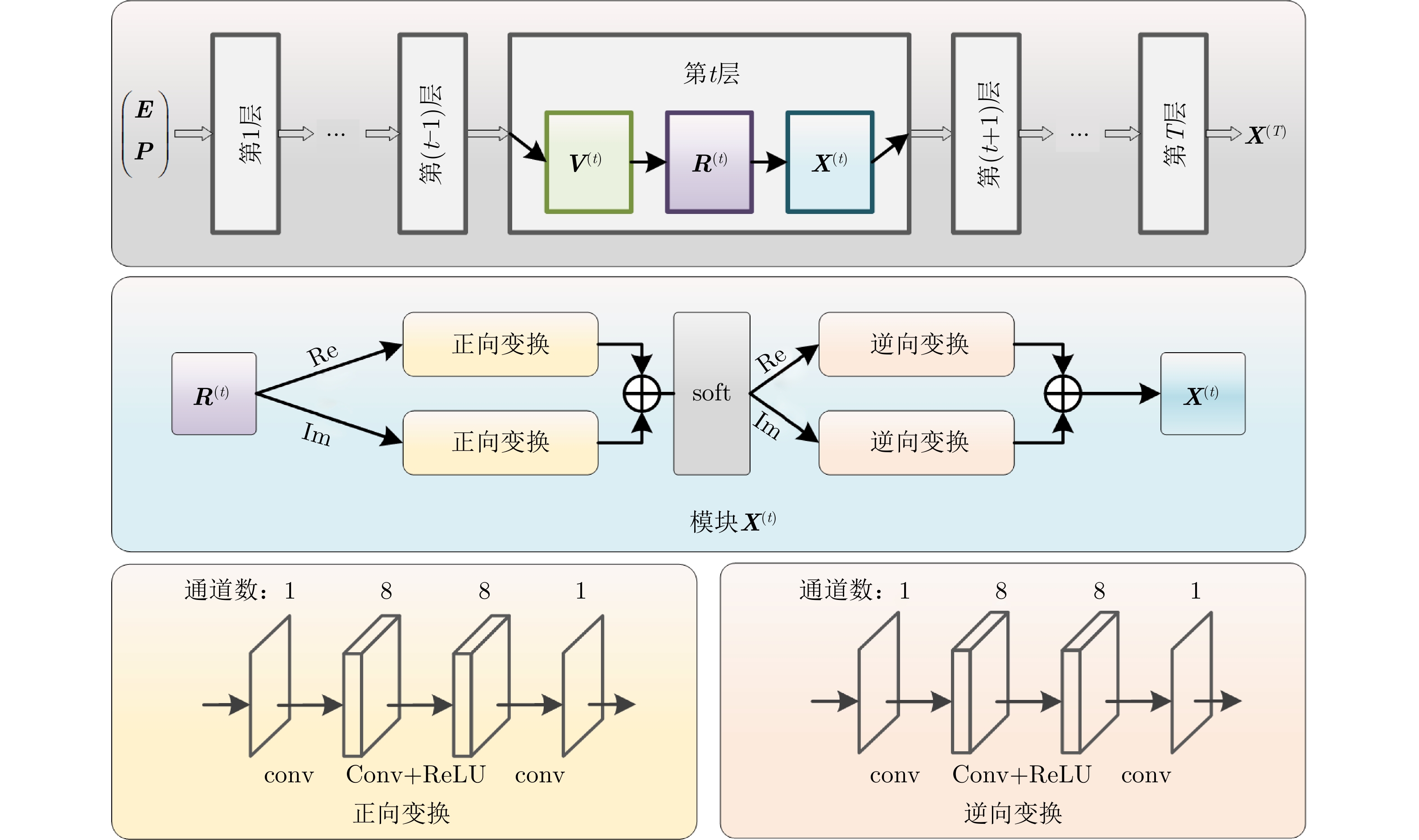
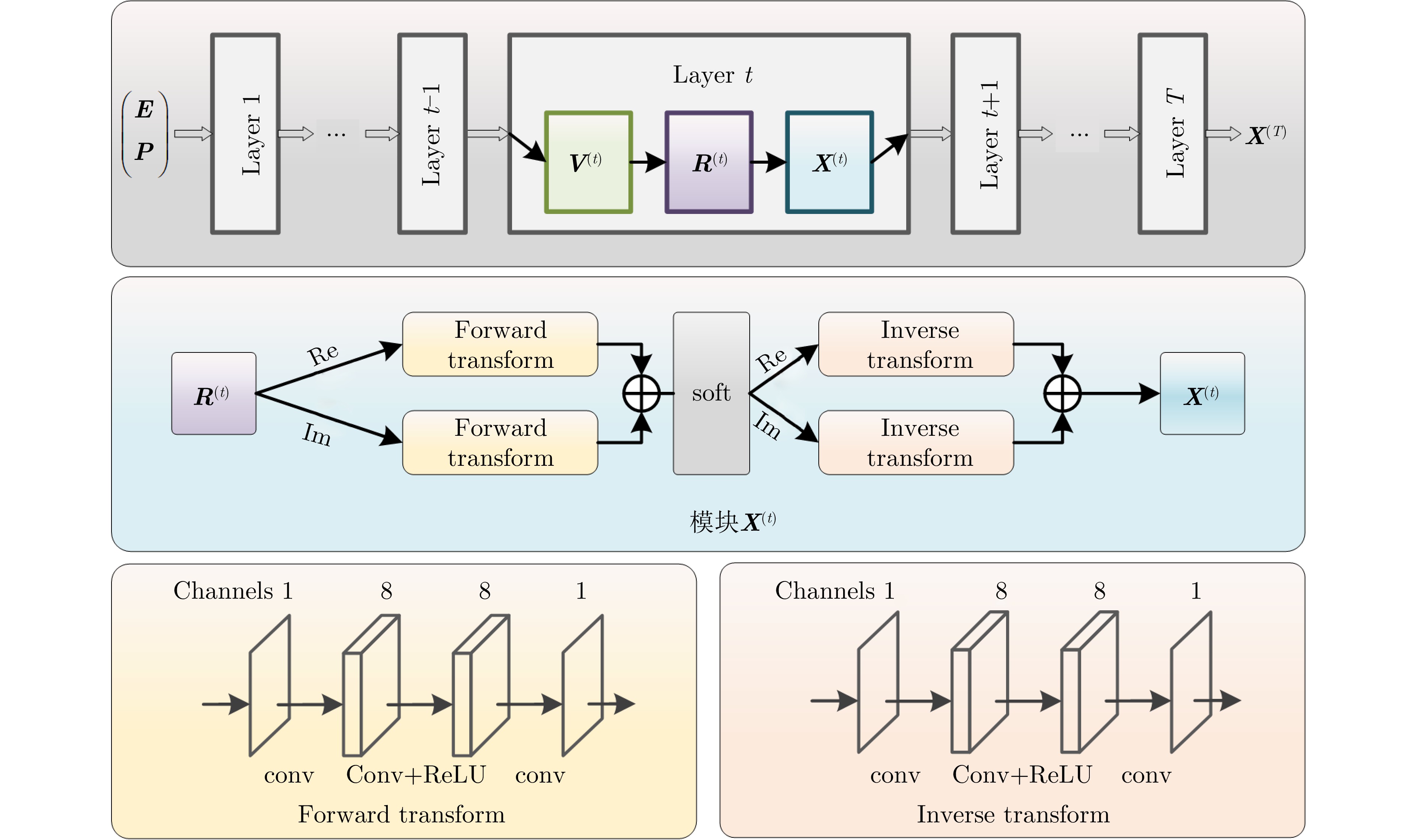
算法2 LSISTA网络稀疏成像算法
Alg. 2 LSISTA network-based sparse imaging algorithm
输入：稀疏降采样回波E，相位传播矩阵P；
输出：稀疏成像结果$ {{\boldsymbol{X}}^{\left( T \right)}} $
初始化：加载卷积核预训练权重，$ \left\{ {{w_1},{b_1},{w_2},{b_2}} \right\} $；
循环开始
(1) 根据式(14)，由$ \left\{ {{w_1},{b_1},{w_2},{b_2}} \right\} $计算$ {\tau ^{\left( t \right)}} $和$ {\lambda ^{\left( t \right)}} $；
(2) 更新迭代残差：$ {{\boldsymbol{V}}^{\left( t \right)}} = {\boldsymbol{E}} - \mathcal{M}\left( {{{\boldsymbol{X}}^{\left( {t - 1} \right)}},{\boldsymbol{\bar P}}} \right) $；
(3) 梯度下降粗估计：$ {{\boldsymbol{R}}^{\left( t \right)}} = {{\boldsymbol{X}}^{\left( {t - 1} \right)}} + {\tau ^{\left( t \right)}}{\mathcal{M}^{\text{H}}}\left( {{{\boldsymbol{V}}^{\left( t \right)}},{\boldsymbol{P}}} \right) $；
(4) 软阈值收缩去噪：　　 ${ {\boldsymbol{X} }^{\left( t \right)} } = \tilde {\mathcal{T} }\left( {{\rm{soft}}} \left( {\mathcal{T}\left( { { {\boldsymbol{R} }^{\left( t \right)} } } \right),{\lambda ^{\left( t \right)} } } \right) \right)$, $t = t + 1$；
(5) 迭代判定：若$t \le T$，则重复步骤(1)—步骤(5)；否则，结束循环。
循环结束

下载: 导出CSV

表 1 各算法在不同采样率情况下的MAE值

Table 1. MAEs of different algorithms in cases of sampling rate being 70% and 30%, respectively

算法	Profile #1		Profile #2		Profile #3
算法	70%	30%	70%	30%	70%	30%
RMA	0.064	0.104	0.075	0.118	0.063	0.105
ISTA	0.024	0.038	0.037	0.058	0.025	0.041
RMIST-Net	0.014	0.022	0.023	0.034	0.015	0.024
LSISTA	0.005	0.012	0.006	0.017	0.005	0.013

下载: 导出CSV

表 2 各算法在不同SNR情况下的MAE值

Table 2. MAEs of different algorithms in cases of SNR being 10 dB and 0 dB, respectively

算法	Profile #1		Profile #2		Profile #3
算法	10 dB	0 dB	10 dB	0 dB	10 dB	0 dB
RMA	0.089	0.118	0.102	0.135	0.085	0.118
ISTA	0.038	0.071	0.056	0.093	0.038	0.072
RMIST-Net	0.018	0.026	0.030	0.046	0.020	0.029
LSISTA	0.005	0.008	0.006	0.015	0.005	0.009

下载: 导出CSV

表 3 仿真和实测系统参数

Table 3. Parameters in simulations and real experiments

参数	三维SAR仿真值	实测系统值
载频(GHz)	77	78.8
带宽(GHz)	4	3.6
孔径尺寸(cm)	100×100	40×40
采样间隔(mm)	x : 7.8; z : 7.8	x : 1; z : 2
距离(m)	15	具体指定

下载: 导出CSV

表 4 三维SAR成像仿真在不同降采样率下各算法的图像熵评估

Table 4. Image entropy of different algorithms with different sampling rates in simulated 3D SAR imaging

算法	50%	30%	Time (s) (CPU/GPU)
RMA	2.757	3.128	0.336/—
ISTA	0.363	0.387	13.561/—
RMIST-Net	0.087	0.062	1.522/0.026
LSISTA	0.299	0.289	7.054/0.033

下载: 导出CSV

表 5 三维SAR成像仿真在信噪比下各算法的图像熵评估

Table 5. Image entropy of different algorithms with different SNRs in simulated 3D SAR imaging

算法	10 dB	0 dB	Time (s) (CPU/GPU)
RMA	2.789	3.155	0.337/—
ISTA	0.548	0.884	14.523/—
RMIST-Net	0.377	0.632	1.630/0.030
LSISTA	0.379	0.419	6.931/0.036

下载: 导出CSV

表 6 图9成像实验中各算法的图像熵评估

Table 6. Image entropy of different algorithms in the experiment of Fig. 9

算法	50%	30%	Time (s) (CPU/GPU)
RMA	4.530	4.761	0.176/—
ISTA	1.125	0.948	6.604/—
RMIST-Net	0.749	0.584	0.156/0.010
LSISTA	0.586	0.429	3.461/0.013

下载: 导出CSV

表 7 图10成像实验中各算法的图像熵评估

Table 7. Image entropy of different algorithms in the experiment of Fig. 10

算法	50%	30%	Time (s) (CPU/GPU)
RMA	6.141	5.960	0.135/—
ISTA	3.567	3.058	6.086/—
RMIST-Net	2.719	2.159	0.115/ 0.009
LSISTA	2.376	1.845	3.103/0.013

下载: 导出CSV

表 8 各算法计算复杂度

Table 8. Computational complexity of different algorithms

算法	FLOPs
RMA	${N_y}{N_s}\left( {10{{\log }_2}{N_s} + 12} \right)$
ISTA	${N_{{\rm{iter}}} }{N_y}{N_s}\left( {10{ {\log }_2}{N_s} + 12} \right)$
RMIST-Net	$ T{N_y}{N_s}\left( {10{{\log }_2}{N_s} + 12} \right) $
LSISTA	$ T{N_s}\left( {{N_y}\left( {10{{\log }_2}{N_s} + 12} \right) + 2846} \right) $

下载: 导出CSV

表 9 各算法在不同目标点数时的MAE评估值

Table 9. MAEs in cases of the different number of target points

目标点数	ISTA	RMIST-Net	LSISTA
99422(37.9%)	0.125	0.121	0.094
24896(9.5%)	0.027	0.026	0.022
6203(2.4%)	0.005	0.005	0.003

下载: 导出CSV

1 ISTA sparse imaging algorithm based on kernel functions.

Input: Sparse undersampled echo E , phase propagation matrix 　 P , iteration step size $\tau $, number of iterations T ;
Output: Sparse imaging result $ {{\boldsymbol{X}}^{\left( T \right)}} $;
Initialization: $t = 1$, ${{\boldsymbol{X}}^{\left( 0 \right)}} = {\mathcal{M}^{\text{H}}}\left( {{\boldsymbol{E}},{\boldsymbol{\bar P}}} \right)$;
For $t = 1,2, \cdots $ do
(1) Update iteration residual： $ {{\boldsymbol{V}}^{\left( t \right)}} = {\boldsymbol{E}} - \mathcal{M}\left( {{{\boldsymbol{X}}^{\left( {t - 1} \right)}},{\boldsymbol{\bar P}}} \right) $;
(2) Gradient descent coarse estimate：　 $ {{\boldsymbol{R}}^{\left( t \right)}} = {{\boldsymbol{X}}^{\left( {t - 1} \right)}} + \tau {\mathcal{M}^{\text{H}}}\left( {{{\boldsymbol{V}}^{\left( t \right)}},{\boldsymbol{P}}} \right) $;
(3) Soft thresholding denoising: $ {{\boldsymbol{X}}^{\left( t \right)}} = {{\mathrm{soft}}} \left( {{{\boldsymbol{R}}^{\left( t \right)}},\lambda } \right) $, 　 $t = t + 1$;
(4) Iteration judgment: if $t \le T$, repeat steps (1)—(4); 　otherwise, end the loop.
End for

下载: 导出CSV

2 LSISTA network-based sparse imaging algorithm.

Input: Sparse undersampled echo E , phase propagation matrix 　 P ;
Output: Sparse imaging result $ {{\boldsymbol{X}}^{\left( T \right)}} $;
Initialization: Load pre-trained convolutional kernel weights $ \left\{ {{w_1},{b_1},{w_2},{b_2}} \right\} $;
For $t = 1,2, \cdots $ do
(1) Calculate $ {\tau ^{\left( t \right)}} $ and $ {\lambda ^{\left( t \right)}} $ based on Eq. (14) using 　 $ \left\{ {{w_1},{b_1},{w_2},{b_2}} \right\} $;
(2) Update iteration residual: $ {{\boldsymbol{V}}^{\left( t \right)}} = {\boldsymbol{E}} - \mathcal{M}\left( {{{\boldsymbol{X}}^{\left( {t - 1} \right)}},{\boldsymbol{\bar P}}} \right) $;
(3) Update iteration residual: 　 $ {{\boldsymbol{R}}^{\left( t \right)}} = {{\boldsymbol{X}}^{\left( {t - 1} \right)}} + {\tau ^{\left( t \right)}}{\mathcal{M}^{\text{H}}}\left( {{{\boldsymbol{V}}^{\left( t \right)}},{\boldsymbol{P}}} \right) $;
(4) Update iteration residual: 　 $ {{\boldsymbol{X}}^{\left( t \right)}} = \tilde {\mathcal{T}}\left( {{{\mathrm{soft}}} \left( {\mathcal{T}\left( {{{\boldsymbol{R}}^{\left( t \right)}}} \right),{\lambda ^{\left( t \right)}}} \right)} \right) $, $t = t + 1$;
(5) Iteration judgment: if $t \le T$, repeat steps (1)—(5); 　otherwise, end the loop.
End for

下载: 导出CSV

表 1 MAEs of different algorithms in cases of sampling rate being 70% and 30%, respectively

Algorithms	Profile #1		Profile #2		Profile #3
Algorithms	70%	30%	70%	30%	70%	30%
RMA	0.064	0.104	0.075	0.118	0.063	0.105
ISTA	0.024	0.038	0.037	0.058	0.025	0.041
RMIST-Net	0.014	0.022	0.023	0.034	0.015	0.024
LSISTA	0.005	0.012	0.006	0.017	0.005	0.013

下载: 导出CSV

表 2 MAEs of different algorithms in cases of sampling rate being 10 and 0 dB, respectively

Algorithms	Profile #1		Profile #2		Profile #3
Algorithms	10 dB	0 dB	10 dB	0 dB	10 dB	0 dB
RMA	0.089	0.118	0.102	0.135	0.085	0.118
ISTA	0.038	0.071	0.056	0.093	0.038	0.072
RMIST-Net	0.018	0.026	0.030	0.046	0.020	0.029
LSISTA	0.005	0.008	0.006	0.015	0.005	0.009

下载: 导出CSV

表 3 Parameters in simulations and real experiments

Parameter	3D SAR simulation value	Real measurement system value
Carrier frequency (GHz)	77	78.8
Bandwidth (GHz)	4	3.6
Aperture size (cm)	100 × 100	40 × 40
Sampling interval (mm)	x: 7.8; z: 7.8	x: 1; z: 2
Range (m)	15	Specified

下载: 导出CSV

表 4 Image entropy of different algorithms with different sampling rates in simulated 3D SAR imaging

Algorithms	50%	30%	Time (s) (CPU/GPU)
RMA	2.757	3.128	0.336/—
ISTA	0.363	0.387	13.561/—
RMIST-Net	0.087	0.062	1.522/ 0.026
LSISTA	0.299	0.289	7.054/0.033

下载: 导出CSV

表 5 Image entropy of different algorithms with different SNRs in simulated 3D SAR imaging

Algorithms	10 dB	0 dB	Time (s) (CPU/GPU)
RMA	2.789	3.155	0.337/—
ISTA	0.548	0.884	14.523/—
RMIST-Net	0.377	0.632	1.630/ 0.030
LSISTA	0.379	0.419	6.931/0.036

下载: 导出CSV

表 6 Image entropy of different algorithms in the experiment of Fig. 9

Algorithms	50%	30%	Time (CPU/GPU)
RMA	4.530	4.761	0.176/—
ISTA	1.125	0.948	6.604/—
RMIST-Net	0.749	0.584	0.156/ 0.010
LSISTA	0.586	0.429	3.461/0.013

下载: 导出CSV

表 7 Image entropy of different algorithms in the experiment of Fig. 10

Algorithms	50%	30%	Time (CPU/GPU)
RMA	6.141	5.960	0.135/—
ISTA	3.567	3.058	6.086/—
RMIST-Net	2.719	2.159	0.115/ 0.009
LSISTA	2.376	1.845	3.103/0.013

下载: 导出CSV

表 8 Computational complexity of different algorithms

Algorithms	FLOPs
RMA	${N_y}{N_s}\left( {10{{\log }_2}{N_s} + 12} \right)$
ISTA	$ {N_{{\mathrm{iter}}}}{N_y}{N_s}\left( {10{{\log }_2}{N_s} + 12} \right) $
RMIST-Net	$ T{N_y}{N_s}\left( {10{{\log }_2}{N_s} + 12} \right) $
LSISTA	$ T{N_s}\left( {{N_y}\left( {10{{\log }_2}{N_s} + 12} \right) + 2846} \right) $

下载: 导出CSV

表 9 MAEs in cases of the different number of target points

Target points	ISTA	RMIST-Net	LSISTA
99422 (37.9%)	0.125	0.121	0.094
24896 (9.5%)	0.027	0.026	0.022
6203 (2.4%)	0.005	0.005	0.003

下载: 导出CSV

参考文献(29)

[1]	杨建宇. 雷达对地成像技术多向演化趋势与规律分析[J]. 雷达学报, 2019, 8(6): 669–692. doi: 10.12000/JR19099. YANG Jianyu. Multi-directional evolution trend and law analysis of radar ground imaging technology[J]. Journal of Radars, 2019, 8(6): 669–692. doi: 10.12000/JR19099.
[2]	吴一戎, 朱敏慧. 合成孔径雷达技术的发展现状与趋势[J]. 遥感技术与应用, 2000, 15(2): 121–123. doi: 10.3969/j.issn.1004-0323.2000.02.012. WU Yirong and ZHU Minhui. The developing status and trends of synthetic aperture radar[J]. Remote Sensing Technology and Application, 2000, 15(2): 121–123. doi: 10.3969/j.issn.1004-0323.2000.02.012.
[3]	CURLANDER J C and MCDONOUGH R N. Synthetic Aperture Radar[M]. New York: Wiley, 1991.
[4]	DONOHO D L. Compressed sensing[J]. IEEE Transactions on Information Theory, 2006, 52(4): 1289–1306. doi: 10.1109/TIT.2006.871582.
[5]	SHI Wuzhen, JIANG Feng, LIU Shaohui, et al. Image compressed sensing using convolutional neural network[J]. IEEE Transactions on Image Processing, 2019, 29: 375–388. doi: 10.1109/TIP.2019.2928136.
[6]	YANG Xianjun, TAO Xiaofeng, DUTKIEWICZ E, et al. Energy-efficient distributed data storage for wireless sensor networks based on compressed sensing and network coding[J]. IEEE Transactions on Wireless Communications, 2013, 12(10): 5087–5099. doi: 10.1109/TWC.2013.090313.121804.
[7]	POTTER L C, ERTIN E, PARKER J T, et al. Sparsity and compressed sensing in radar imaging[J]. Proceedings of the IEEE, 2010, 98(6): 1006–1020. doi: 10.1109/JPROC.2009.2037526.
[8]	CAMLICA S, GURBUZ A C, and ARIKAN O. Autofocused spotlight SAR image reconstruction of off-grid sparse scenes[J]. IEEE Transactions on Aerospace and Electronic Systems, 2017, 53(4): 1880–1892. doi: 10.1109/TAES.2017.2675138.
[9]	PU Wei and WU Junjie. OSRanP: A novel way for radar imaging utilizing joint sparsity and low-rankness[J]. IEEE Transactions on Computational Imaging, 2020, 6: 868–882. doi: 10.1109/TCI.2020.2993170.
[10]	DONOHO D L, MALEKI A, and MONTANARI A. Message-passing algorithms for compressed sensing[J]. Proceedings of the National Academy of Sciences of the United States of America, 2009, 106(45): 18914–18919. doi: 10.1073/pnas.0909892106.
[11]	BOYD S, PARIKH N, CHU E, et al. Distributed optimization and statistical learning via the alternating direction method of multipliers[J]. Foundations and Trends® in Machine Learning, 2011, 3(1): 1–122. doi: 10.1561/2200000016.
[12]	BECK A and TEBOULLE M. A fast iterative shrinkage-thresholding algorithm for linear inverse problems[J]. SIAM Journal on Imaging Sciences, 2009, 2(1): 183–202. doi: 10.1137/080716542.
[13]	ZHAO Lifan, WANG Lu, YANG Lei, et al. The race to improve radar imagery: An overview of recent progress in statistical sparsity-based techniques[J]. IEEE Signal Processing Magazine, 2016, 33(6): 85–102. doi: 10.1109/MSP.2016.2573847.
[14]	FANG Jian, XU Zongben, ZHANG Bingchen, et al. Fast compressed sensing SAR imaging based on approximated observation[J]. IEEE Journal of Selected Topics in Applied Earth Observations and Remote Sensing, 2014, 7(1): 352–363. doi: 10.1109/JSTARS.2013.2263309.
[15]	JIANG Chenglong, ZHANG Bingchen, FANG Jian, et al. Efficient ℓq regularisation algorithm with range–azimuth decoupled for SAR imaging[J]. Electronics Letters, 2014, 50(3): 204–205. doi: 10.1049/el.2013.1989.
[16]	GREGOR K and LECUN Y. Learning fast approximations of sparse coding[C]. The 27th International Conference on International Conference on Machine Learning, Haifa, Israel, 2010: 399–406.
[17]	PU Wei. SAE-Net: A deep neural network for SAR autofocus[J]. IEEE Transactions on Geoscience and Remote Sensing, 2022, 60: 5220714. doi: 10.1109/TGRS.2021.3139914.
[18]	WANG Mou, WEI Shunjun, SHI Jun, et al. CSR-Net: A novel complex-valued network for fast and precise 3-D microwave sparse reconstruction[J]. IEEE Journal of Selected Topics in Applied Earth Observations and Remote Sensing, 2020, 13: 4476–4492. doi: 10.1109/JSTARS.2020.3014696.
[19]	HU Xiaowei, XU Feng, GUO Yiduo, et al. MDLI-Net: Model-driven learning imaging network for high-resolution microwave imaging with large rotating angle and sparse sampling[J]. IEEE Transactions on Geoscience and Remote Sensing, 2021, 60: 5212617. doi: 10.1109/TGRS.2021.3110579.
[20]	WEI Yangkai, LI Yinchuan, DING Zegang, et al. SAR parametric super-resolution image reconstruction methods based on ADMM and deep neural network[J]. IEEE Transactions on Geoscience and Remote Sensing, 2021, 59(12): 10197–10212. doi: 10.1109/TGRS.2021.3052793.
[21]	WEI Shunjun, LIANG Jiadian, WANG Mou, et al. AF-AMPNet: A deep learning approach for sparse aperture ISAR imaging and autofocusing[J]. IEEE Transactions on Geoscience and Remote Sensing, 2021, 60: 5206514. doi: 10.1109/TGRS.2021.3073123.
[22]	WANG Mou, WEI Shunjun, ZHOU Zichen, et al. Efficient ADMM framework based on functional measurement model for mmW 3-D SAR imaging[J]. IEEE Transactions on Geoscience and Remote Sensing, 2022, 60: 5226417. doi: 10.1109/TGRS.2022.3165541.
[23]	WANG Mou, WEI Shunjun, LIANG Jiadian, et al. TPSSI-Net: Fast and enhanced two-path iterative network for 3D SAR sparse imaging[J]. IEEE Transactions on Image Processing, 2021, 30: 7317–7332. doi: 10.1109/TIP.2021.3104168.
[24]	PU Wei. Deep SAR imaging and motion compensation[J]. IEEE Transactions on Image Processing, 2021, 30: 2232–2247. doi: 10.1109/TIP.2021.3051484.
[25]	WANG Mou, WEI Shunjun, LIANG Jiadian, et al. Lightweight FISTA-inspired sparse reconstruction network for mmW 3-D holography[J]. IEEE Transactions on Geoscience and Remote Sensing, 2021, 60: 5211620. doi: 10.1109/TGRS.2021.3093307.
[26]	WANG Mou, WEI Shunjun, LIANG Jiadian, et al. RMIST-Net: Joint range migration and sparse reconstruction network for 3-D mmW imaging[J]. IEEE Transactions on Geoscience and Remote Sensing, 2021, 60: 5205117. doi: 10.1109/TGRS.2021.3068405.
[27]	ZHANG Jian and GHANEM B. ISTA-Net: Interpretable optimization-inspired deep network for image compressive sensing[C]. The 2018 IEEE/CVF Conference on Computer Vision and Pattern Recognition, Salt Lake City, USA, 2018: 1828–1837.
[28]	ZHOU Yulong, ZHONG Yu, WEI Zhun, et al. An improved deep learning scheme for solving 2-D and 3-D inverse scattering problems[J]. IEEE Transactions on Antennas and Propagation, 2021, 69(5): 2853–2863. doi: 10.1109/TAP.2020.3027898.
[29]	LOPEZ-SANCHEZ J M and FORTUNY-GUASCH J. 3-D radar imaging using range migration techniques[J]. IEEE Transactions on Antennas and Propagation, 2000, 48(5): 728–737. doi: 10.1109/8.855491.