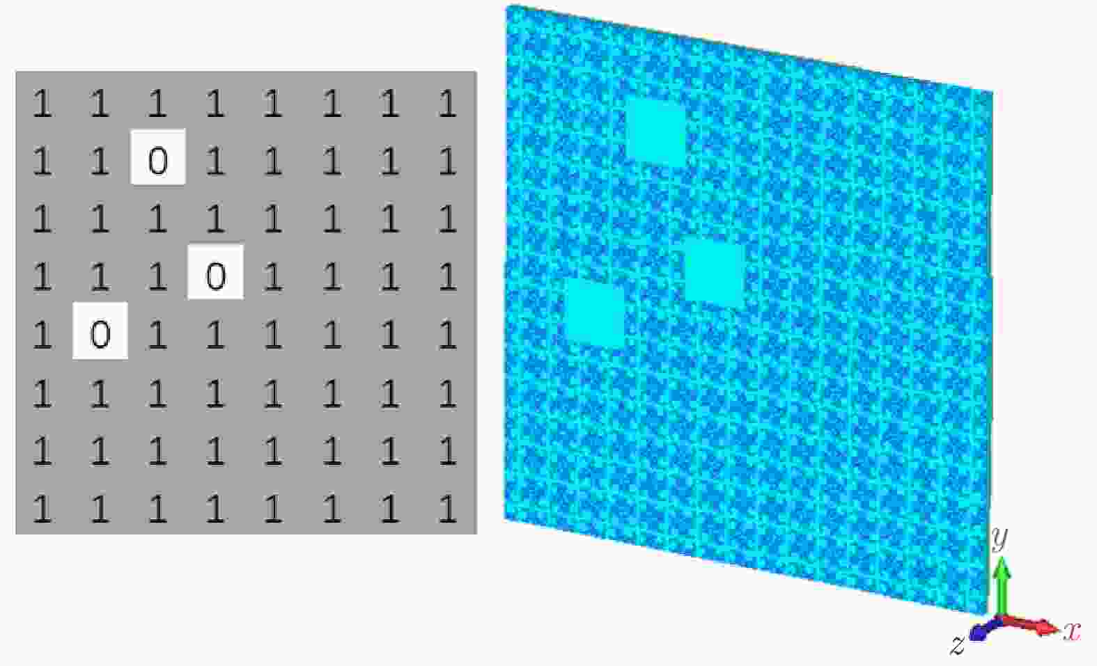
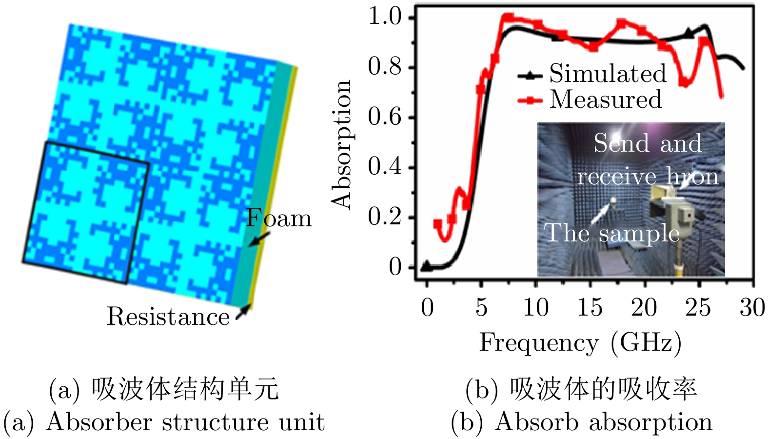
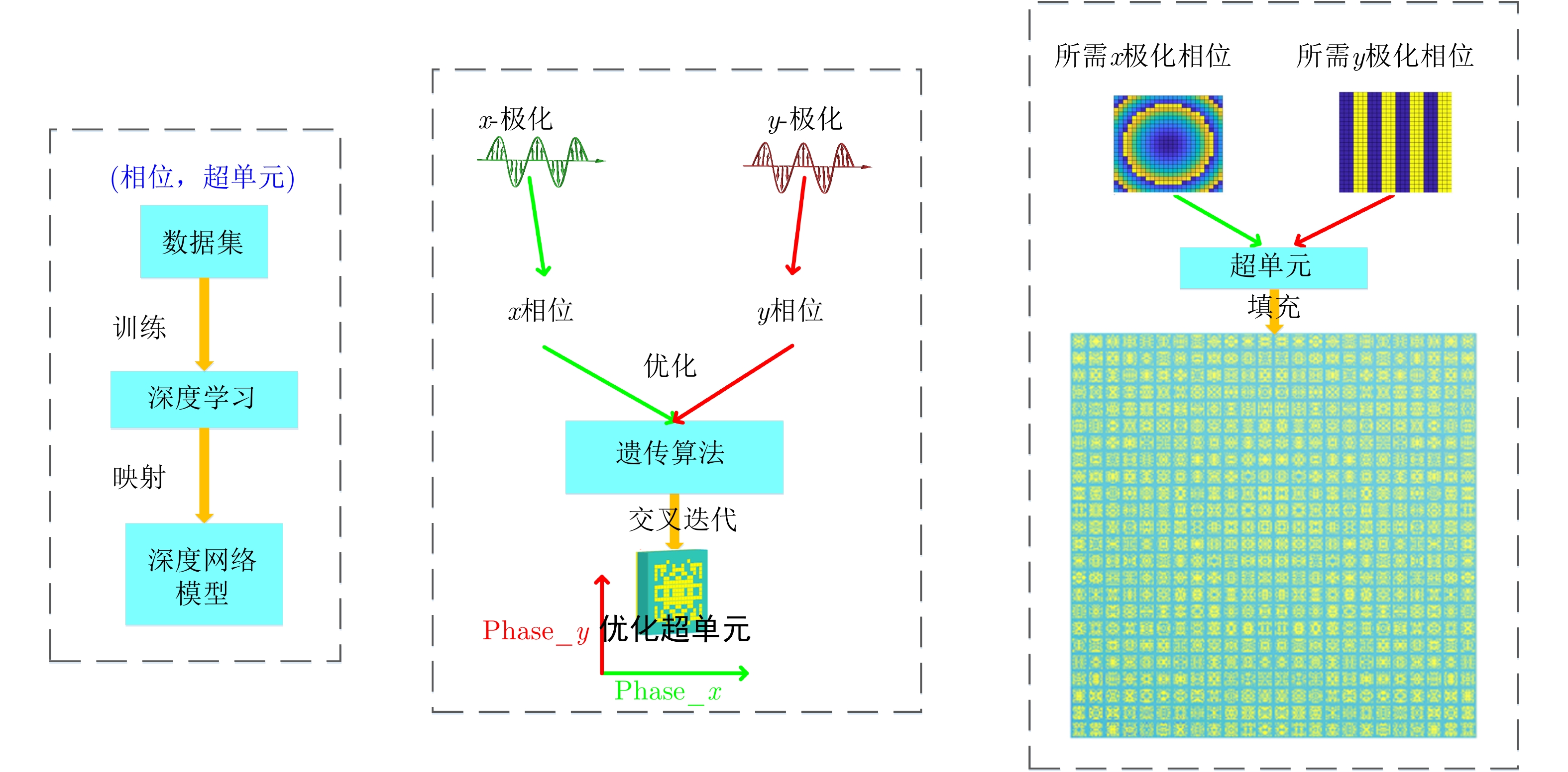
1. Introduction

High resolution radar imaging has been widely used in target scattering diagnostics and recognition. As we all know, high resolution in range dimension is derived from the bandwidth of the transmitting signal and in the cross range dimension from synthetic aperture of multiple spatial positions. Under the fixed bandwidth and the synthetic aperture, traditional Matched Filter (MF) based methods for radar imaging suffer from low resolution and high sidelobes limited by the synthetic aperture^[1].

In order to improve the resolution and suppress the sidelobes, many high resolution methods have been applied to radar imaging. For example, the recently introduced theory of Compressed Sensing (CS) provides an idea to improve the resolution and reduce the amounts of measurement data under the constraint of sparsely distributed target prior, which has been widely explored for applications of radar imaging^[2–4]. However, conventional CS methods are confronted with a range of problems in practical scenarios, such as complexity in calculation, high Signal-to-Noise Ratio (SNR) requirement, model mismatch caused by off grid problem^[5], phase mismatch^[6], frequency error^[7] and position error^[8]. To avoid the off grid problem of CS, modern spectral estimation methods like MUltiple SIgnal Classification (MUSIC), matrix pencil and Estimation of Signal Parameters via Rotational Invariance Techniques (ESPRIT) have been used in radar imaging for resolution improvement^[9]. However, most those methods suffer from performance degradation when there is little prior knowledge of the exact numbers of the scatters or under low SNR condition. Recently, the atomic norm minimization algorithm^[10] based on continuous compressed sensing is introduced to enhance the SNR of the received echo and using Vandermonde decomposition to eliminate the grid mismatch. Nevertheless, this method can only be tailored to a specific model and brings huge computational cost.

Consideration the aforementioned fact while combining the sparsity low rank matrix recovery technology and deconvolution algorithm, we introduce a high resolution radar imaging method based on the MF result. Firstly we establish the convolution model of target’s backscatter coefficients and the Point Spread Function (PSF), and then we want to use the deconvolution method like Wiener filter to improve the radar imaging resolution. However, the performance improvements of those methods depend on high SNR, and their super resolution performance is visibly affected by the low pass character of the PSF^[11]. Although the MF result has enhanced the SNR, we can further improve the echo SNR by the sparsity and low rank matrix recovery. Low rank matrix recovery has been applied in many signal processing applications to estimate a low rank matrix from its noisy observation^{[12, 13]}. Combinng the sparsity of the echo matrix, we modify the low rank matrix recovery and introduce it to radar echo denoising, which can improve the performance of the two-Dimensional (2D) deconvolution. Finally, some experimental results are conducted to verify the effectiveness of the proposed method.

Notation: (·)^T, (·)^H and (·)^* denote the transpose, the conjugate transpose and the conjugate operation, respectively. $\left\langle \cdot \right\rangle$,﹡, and ☉ indicate the inner product, the convolution and the Hadamard product. ${\left\| \cdot \right\|_F}$, ${\left\| \cdot \right\|_1}$, ${\left\| \cdot \right\|_ * }$ are the Frobenius norm, sum of the absolute values and the nuclear norm.

2. Model Establishment

Considering a typical arrangement for radar imaging in which an object with scattering reflectivity ${\sigma _{xy}}$ rotated by a scan angle ${\theta _m}$ (as shown in Fig. 1), we defined the positions of the transmitting and receiving antenna shown in a Cartesian coordinate as (W/2, –R, H) and (–W/2, –R,H), where W, R, H represent the antenna spacing, distance from antenna to XZ plane and XY plane, respectively.

Figure  1.  Radar imaging geometry

DownLoad: Full-Size Img PowerPoint

Transmitting a stepped-frequency signal with frequency ${f_{\!n}}$ and under Born approximation, the received scattered echo with Gauss noise W_mn is given by:

In this equation: ${f_{\!n}} = {f_0} + n\Delta f,n = 0,1 ·\!·· ,N - 1$, ${f_0}$ and $\Delta f$ represent the start frequency and frequency step, ${\theta _m} = m\Delta \theta ,m = 0,1, ·\!·\!· ,M$, $\Delta \theta$ represents the rotating angle step, respectively. The range $R\left( {x,y;{\theta _m}} \right)$ from the transmitting antenna to echo scattering center and to the receiving antenna can be calculated as Eq. (2):

In far-field and small rotation angle case, $R\left( {x,y;{\theta _m}} \right)$ can be approximated by first order Taylor-series expansion as:

where ${R_0} = \sqrt {{R^2} + {{\left( {W/2} \right)}^2} + {H^2}}$.

Then the received echo can be written as follow under some approximated conditions:

where ${\tilde \sigma _{xy}} \!\!=\!\! {\sigma _{xy}}{{\rm{e}}^{ - {\rm{j}}4{\text{π}} Ry/\!\lambda {R_0}}}$, $\;\;{{{\tilde Y} }_{mn}} \!\!=\!\!\! {Y_{mn}}{{\rm{e}}^{{\rm{j}}4{\text{π}} {f_{\!n}}{R_0}/\!c}}$, $\lambda \!\!\approx\!\! c/\!{f_0}$.

After discrete imaging region with P×Q grids, the received echo in Eq. (4) can be described as the following 2D linear signal model:

where ${\tilde{\text{Y}}} \!\!=\!\! {\left[ \ \ {{{\tilde {Y}}_{mn}}} \right]_{M \times N}}$ is the echo matrix, $\tilde{{\text{Σ}} } \!=\! {\left[ {{{\tilde \sigma }_{pq}}} \right]_{P \times Q}}$ is the observation matrix: ${{{\text{A}}}_x} = {\left[ {{{\rm{e}}^{ - {\rm{j}}4{\text{π}} m{x_p}R\Delta \theta /\lambda {R_0}}}} \right]_{M \times P}}$, ${{{\text{A}}}_y} = {\left[ {{{\rm{e}}^{ - {\rm{j}}4{\text{π}} n{y_q}R\Delta f/{R_0}c}}} \right]_{N \times Q}}$.

Considering the targets present sparse point scattering characteristic under high frequency scattering in most practical application scenarios, we present our method to improve the resolution of radar imaging under sparse target constraint using 2D deconvolution algorithm with low rank sparsity echo matrix denoising.

3. 2D Deconvolution with Echo Denoising

As we all know, the MF algorithm which is based on the maximum signal to noise ratio is the most stable and commonly used radar imaging method. However, due to limitation of the synthetic aperture and bandwidth, the standard MF method suffers from relatively low resolution and high sidelobes, especially under the requirements of high resolution. The received echo after MF from Eq. (5) can be obtained by:

From the result of Eq. (6), the echo of the surface target after MF can be described as the sum of all the wave scattered at the points on the surface grid, i.e.,

where we define the PSF as:

here, ${{\text{a}}_x}\left( x \right)$ and ${{\text{a}}_y}\left( y \right)$ represent the column of matrix A_x and A_y at the grid (x, y).

We can find that Eq. (6) can be seen as the 2D convolution of the PSF and target backscatter coefficients:

Inspired by this, we can recovery the backscatter coefficients using deconvolution algorithm to improve the imaging quality. Firstly, we should analyze the characteristic of the PSF and its influence on the deconvolution result.

3.1 Analysis of PSF

The PSF can be evaluated as:

(10)

We can calculate the 2D mainlobe width which represents the radar imaging resolution as follows:

Eq. (9) indicates that the MF result can be seen as the convolution result of backscatter coefficients and ${P_{sf}}\left( {x,y} \right)$. The PSF is characterized by synthetic aperture and bandwidth, which has strong low pass characteristic with low resolution and high sidelobes as shown in Eq. (10) and Eq. (11). For an isolated target scatter, imaging result after the MF output will be proportional to the PSF, therefore the resolution of MF result is limited and accompanied by low resolution and high sidelobes. Inspired by above, we can restore the high resolution backscatter coefficients information by deconvolution to remove the effect of low pass characteristic of PSF.

3.2 2D deconvolution

As we have get 2D convolution form as Eq. (9), here we consider to use the direct deconvolution algorithm to recovery target backscatter coefficients. Firstly, we transform Eq. (9) into the spatial frequency domain using 2D Fourier transform as:

where, ${{{\text{Y}}}_{\!\omega} } \!=\!\! \mathcal{F}\left\{ {{{{\text{Y}}}_{\!\!{\rm {MF}}}}} \right\},{{\text{Σ}}_\omega } \!=\!\! \mathcal{F}\left\{ {\tilde{{\text{Σ}} }} \right\},{{{\text{H}}}_\omega } \!=\!\! \mathcal{F}\left\{ {{{{\text{P}}}_{\!\!sf}}} \right\},$${{{\text{W}}}_{\!\!\omega} } \!=\! \mathcal{F}\left\{ {{{{\text{W}}}_{\!\!{\rm {MF}}}}} \right\}$.

Theoretically, the target scattering information could be restored by deconvolution as:

However, $1/{{{\text{H}}}_\omega }$ will be very large in practice at the outside of the mainlobe of PSF since the low pass characteristic of the PSF, which results in tremendous amplification of noise and obtains valueless results. So the deconvolution processing becomes an ill-posed inverse problem.

In order to alleviate the ill-posed problem, we use Winner filtering algorithm and sparse low rank matrix recovery to improve the quality of imaging result.

The result after Winner filter algorithm can be written as^[14]:

where ${\Psi _{\rm WW}}\left( \omega \right)$ and ${\Psi _{\Sigma \Sigma }}\left( \omega \right)$ is the power spectral density of ${{\text{W}}}$ and ${\text{Σ}}$. Eq. (14) will approach Eq. (13) when the SNR is relatively high. What’s more, Eq. (14) will attenuate the high frequencies noise to alleviate the ill-posed problem under low SNR. In experimental data processing, the ${\Psi _{\rm WW}}\left( \omega \right)/{\Psi _{\Sigma \Sigma }}\left( \omega \right)$ is generally set according to the experience value. We can get the scattering reflectivity $\tilde{{\text{Σ}} }$ by 2D Inverse Fourier transform according to Eq. (14).

3.3 Echo denoising by sparse low rank matrix recovery

We can prove that the echo matrix after MF is sparse and low rank in Appendix A and by using this characteristic, the echo SNR can be improved. Consider the problem of estimating a sparse low rank matrix X from its noisy observation Y:

Define the sparse low rank matrix recovery problem as:

where $\gamma$ is the regularization parameter used to balance the relative contribution between nuclear norm and the 1-norm, which can control the denoising performance. In general, the denoising threshold of $\gamma$ can be set as the 5%～10% of the maximum singular value of Y.

By applying Augmented Lagrangian Method (ALM), we can get the optimization problem:

(17)

And the update rules for solving this problem are as follows:

where, $\mathcal{S}\left( { \cdot , \cdot } \right)$ is the singular value thresholding function defined as:

where, ${{\text{X}}} = {{\text{U}}}{\text{Σ}}{{{\text{V}}}^{\rm T}\,}$ is the Singular Value Decomposition (SVD) of ${{\text{X}}}$, ${\rm{soft}}\left( \cdot \right)$ is the soft thresholding function defined as:

See Appendix B for the detailed derivation of Eq. (18) and Eq. (19).

The flowchart of the proposed method is shown in Fig. 2 by combining the sparse low rank matrix recovery with the 2D deconvolution.

Figure  2.  The flowchart of the proposed method

DownLoad: Full-Size Img PowerPoint

4. Simulation

The parameters in the simulation are given in Tab. 1. In this experiment, we set four-point targets, the imaging results are shown in Fig. 3.

Table  1.  Simulation parameters

Parameter	Value	Parameter	Value
${{M}}$	256	$R$	1 m
${{N}}$	500	$H$	0.7 m
$\Delta f$	10 MHz	W	0.04 m
$\Delta \theta$	0.009°	SNR	–15 dB

 | Show Table

DownLoad: CSV

Figure  3.  Imaging results

DownLoad: Full-Size Img PowerPoint

As shown in Fig. 3(a), due to the limitation of synthetic aperture and bandwidth, the MF method suffers from relatively low resolution and high sidelobes which make it difficult to distinguish between four-point targets even there is no noise. Fig. 3(b)–Fig. 3(d) show the imaging results reconstructed by MF and proposed method including the intermediate denoising results when SNR = –15 dB. It can be clearly seen that the effect of denoising compared Fig. 3(c) with Fig. 3(a) and Fig. 3(b), the echo SNR is further improved by the sparsity and low rank matrix recovery during the proposed intermediate denoising procedure. The final imaging result is shown in Fig. 3(d), from which we can see that the proposed method has a better reconstruction precision with higher resolution imaging of four distinguishable point targets.

5. Experiment Results

The experimental scene is shown in Fig. 4(a), which is the same with the model in Fig. 1. The radar system consists of a pair of horn antennas, a turntable whose rotation angle can be precisely controlled by the computer, and an Agilent VNA N5224A which is used for transmitting and receiving the stepped-frequency signal with bandwidth of 10 GHz from 28 GHz to 38 GHz and number of frequencies N equals to 256 (Frequency interval $\Delta$f is 40 MHz). Two kind of targets including three 5-mm-diameter mental spheres and a pair of scissors placed on a rotatory platform are used here as shown in Fig. 4(b).

Figure  4.  Experimental scene VNA

DownLoad: Full-Size Img PowerPoint

As we know, image entropy can be considered as a metric for measuring the smoothness of the probability density function of image intensities^[15]. The imaging entropy is defined as:

where $s\left( I \right) = \displaystyle\sum\nolimits_{p = 1}^P {\sum\nolimits_{q = 1}^Q {{{\left| {I\left( {p,q} \right)} \right|}^2}} }$.

5.1 Three mental spheres

In this experiment, we set $R \!=\! 1\;{\rm m},\ H \!=\! 0.7\;{\rm m},$$W = 0.04\;{\rm m}$ and the total rotating angle is ${5^ \circ }$ with an angle interval $\Delta \theta = {0.01^ \circ }$ ($M = 500$).

Fig. 5 shows the results of the MF and our proposed method for the mental spheres. The one-dimensional $x$ and $y$ domain cross-section of the target with red-dashed circle shown in Fig. 5 are presented in Fig. 6, in which the red-dashed line and blue line represent the result of MF and proposed method. Clearly, the reconstruction result of proposed method has a narrower main-lobe and lower side-lobe than MF and the sharpening ratio almost reach 5.8 and 3.0 in $x$ and $y$ domain, respectively.

Figure  5.  Imaging results of mental spheres

DownLoad: Full-Size Img PowerPoint

Figure  6.  One-dimensional cut through the target with red dashed circle in Fig. 5

DownLoad: Full-Size Img PowerPoint

5.2 Scissors

The parameters for this experiment are set as follows, $R = 0.876\;{\rm m}$, $W = 0.04\;{\rm m}$. The total rotating angle is ${360^ \circ }$ with $M$ equals to ${720^ \circ }$. Taking into account the scintillation characteristics of the target under large rotating angle, we divide the rotating angle into 72 segments and each of the part is with rotating angle from ${0^ \circ }$ to ${5^ \circ }$. The proposed method is used to process the data for each segment and the image fusion method is used to merge the results of all segments.

Fig. 7 shows the imaging results of the scissors reconstructed by MF and proposed method. It can be seen from the results that the proposed method has a high reconstruction precision with a shaper shape of scissors.

Figure  7.  Imaging results of scissors

DownLoad: Full-Size Img PowerPoint

The entropies of the imaging results by MF and our proposed method are given in Tab. 2 to quantitatively assess the performance. The proposed method has a low entropy which means the proposed method can improve the resolution and verifies its superiority.

Table  2.  Entropies of imaging results

Target	MF	Our proposed method
Mental spheres	8.7282	4.8429
Scissors	8.9433	7.0454

 | Show Table

DownLoad: CSV

6. Conclusion

We introduce a robust deconvolution method with enhancing SNR technology to realize high resolution radar imaging. Compared to other high resolution methods, our proposed method is simple and robust. Although the signal model and experiments are performed for turntable radar situation with SF waveform, the method can be directly generalized to other practical radar systems based on other types of signals.

Appendix A Proof of the sparsity and low rank characteristic

To prove the echo matrix after MF is sparse and low rank, the following lemma is needed.

Lemma 1^[16]: For matrix A and B, the ranks of the product of A and B satisfy the inequality below:

From Eq. (5) and Eq. (6), we can see that the echo matrix after MF can be written as:

We have supposed that the target has sparse distribution, so the target backscatter coefficients matrix $\tilde{{\text{Σ}} }$ is sparse and low rank. Thus, matrix ${{{\text{Y}}}_{{\!\rm{MF}}}}$ is also low rank according to lemma 1. The sparsity of matrix ${{{\text{Y}}}_{{\rm{\!\!MF}}}}$ can be proved by Eq. (9) obviously.

Appendix B Derivation of Eq. (18) and Eq. (19)

For Eq. (18), the optimization problem can be described as Eq. (B-1), and it has a closed-form solution just as Eq. (18) according to Ref. [13].

For Eq. (19), it is the same with Eq. (18), which can written as

It also has a closed-form solution as Eq. (19) according to Ref. [17].