基于特征复用的膨胀-残差网络的SAR图像超分辨重建

李萌; 刘畅

doi:10.12000/JR19110

基于特征复用的膨胀-残差网络的SAR图像超分辨重建

DOI: 10.12000/JR19110

李萌,
刘畅^,

1.
中国科学院空天信息创新研究院北京 100190
2.
中国科学院电子学研究所北京 100190
3.
中国科学院大学北京 100049

基金项目: 国家重点研发计划(2017YFB0503001)

详细信息

作者简介:
李　萌(1994–)，女，甘肃庆阳人，中国科学院大学硕士研究生，研究方向为SAR图像处理、机器学习。E-mail: limeng173@mails.ucas.ac.cn

刘　畅(1978–)，男，山东烟台人，研究员，博士生导师。2006年在中国科学院电子学研究所获得博士学位，现担任中国科学院空天信息创新研究院研究员、博士生导师。主要研究方向为SAR系统及其相关SAR成像处理。E-mail: cliu@mail.ie.ac.cn

通讯作者:
刘畅 cliu@mail.ie.ac.cn

责任主编：李宁 Corresponding Editor: LI Ning
中图分类号: TN958
计量
- 文章访问数: 3737
- HTML全文浏览量: 1249
- PDF下载量: 574
- 被引次数: 10
出版历程
- 收稿日期: 2019-12-06
- 修回日期: 2020-03-05
- 网络出版日期: 2020-04-01

Super-resolution Reconstruction of SAR Images Based on Feature Reuse Dilated-Residual Convolutional Neural Networks

LI Meng,
LIU Chang^,

1.
Aerospace Information Research Institute, Chinese Academy of Sciences, Beijing 100190, China
2.
Institute of Electronics, Chinese Academy of Sciences, Beijing 100190, China
3.
University of Chinese Academy of Sciences, Beijing 100049, China

Funds: The State Key Research Development Program of China (2017YFB0503001)

More Information

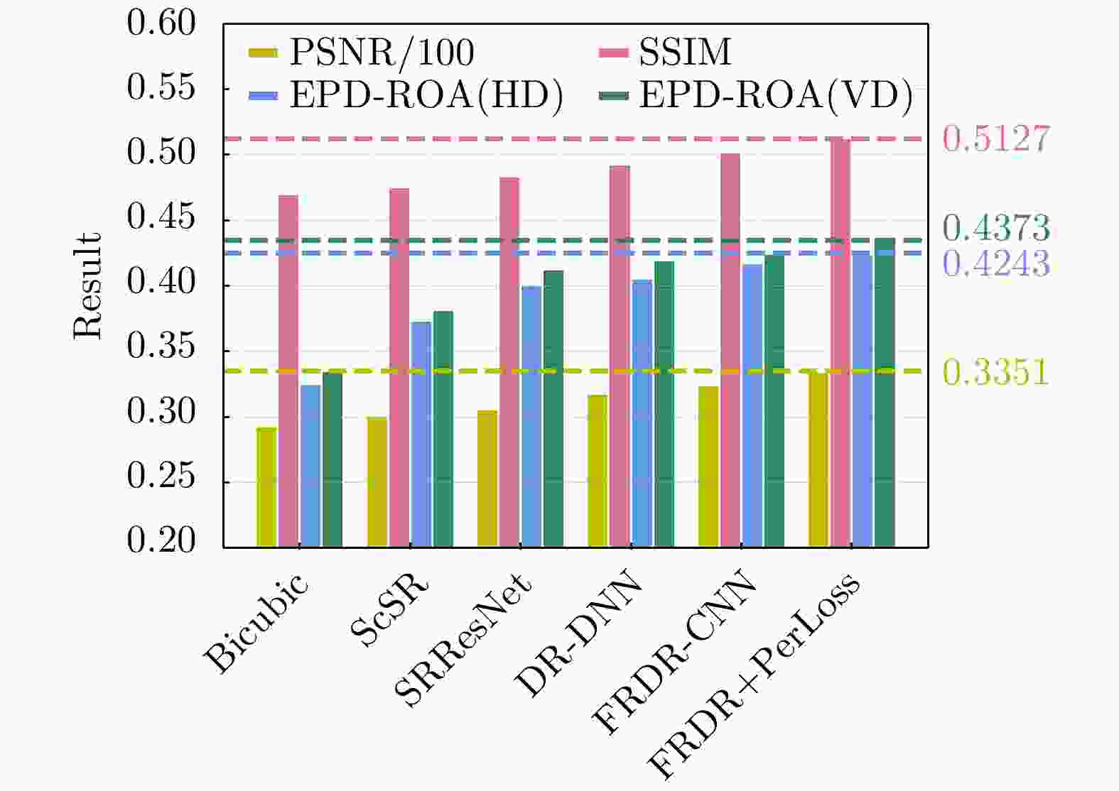
Corresponding author: LIU Chang, cliu@mail.ie.ac.cn

摘要

摘要: 对于合成孔径雷达(SAR)图像，传统的超分辨重建方法对视觉特征的人为构造十分依赖，基于普通卷积神经网络(CNN)的超分辨重建方法对微小目标的重建能力较弱，对边缘轮廓的保真度较差。针对以上问题，该文提出一种基于特征复用的膨胀-残差卷积超分辨网络模型，同时引入感知损失，实现了精确的SAR图像4倍语义级超分辨。该方法为增加网络感受野，采用膨胀-残差卷积(DR-CNN)结构用于限制模型中特征图分辨率的严重损失，提高网络对微小细节的敏感度；为实现不同层级的特征最大化利用，将不同层级的特征图进行级联，形成一种特征复用结构(FRDR-CNN)，以此大幅度提升特征提取模块的效率，进一步提升超分辨精度；针对SAR图像特殊的相干斑噪声干扰，引入感知损失，使得该方法在恢复图像边缘和精细的纹理信息方面具有优越表现。文中实验表明，与传统算法以及目前较为流行的几种全卷积神经网络超分辨重建算法相比，该文采用的FRDR-CNN模型在视觉上对小物体的超分辨重建能力更强，对边界等轮廓信息的重建更准确，客观指标中的峰值信噪比(PSNR)和结构相似性指数(SSIM)分别为33.5023 dB和0.5127，边缘保持系数(EPD-ROA)在水平和垂直方向上分别为0.4243和0.4373。
- 合成孔径雷达 /
- 超分辨重建 /
- 膨胀卷积 /
- 特征复用 /
- 感知损失
Abstract: For Synthetic Aperture Radar (SAR) images, traditional super-resolution methods heavily rely on the artificial design of visual features, and super-reconstruction algorithms based on general Convolutional Neural Network (CNN) have poor fidelity to the target edge contour and weak reconstruction ability to small targets. Aiming at the above problems, in this paper, a Dilated-Resnet CNN (DR-CNN) super-resolution model based on feature reuse, i.e., Feature Reuse Dilated-Resnet CNN (FRDR-CNN), is proposed and perceptual loss is introduced, which accurately realizes four times the semantic super-resolution of SAR images. To increase the receptive field, a DR-CNN structure is used to limit the serious loss of the feature map’s resolution in the model, improving the sensitivity to tiny details. To maximize the utilization of features at different levels, the FRDR-CNN cascades the feature maps of different levels, which greatly improves the efficiency of the feature extraction module and further improves the super-resolution accuracy. With the introduction of the perceptual loss, this method has a superior performance in recovering image texture and edge information. Experimental results of the study show that the FRDR-CNN algorithm is more capable of providing small objects’ super-resolution and more accurate in the visual reconstruction of contour details, compared with traditional algorithms and several popular CNN super-resolution algorithms. Objectively, the Peak Signal to Noise Ratio (PSNR) is 33.5023 dB and Structural Similarity Index (SSIM) is 0.5127, and the Edge Preservation Degreebased on the Ratio Of Average (EPD-ROA) is 0.4243 and 0.4373 in the horizontal and vertical directions, respectively.
- SAR /
- Super resolution construction /
- Dilated convolution /
- Feature reuse /
- Perceptual loss

HTML全文

1. Introduction

In recent years, Frequency Diverse Array (FDA) radar has received much attention due to its range-angle-time-dependent beampattern^[1,2]. Combining the advantages of FDA and traditional phased array Multiple-Input Multiple-Output (MIMO) radar in the degree of freedom, the FDA Multiple-Input Multiple Output (FDA-MIMO) radar was proposed in Ref. [3] and applied in many fields^[4-9]. For parameter estimation algorithm, the authors first proposed a FDA-MIMO target localization algorithm based on sparse reconstruction theory^[10], and an unbiased joint range and angle estimation method was proposed in Ref. [11]. The work of Ref. [12] further proved that the FDA-MIMO is superior to traditional MIMO radar in range and angle estimation performance, and the authors of Ref. [13] introduced a super-resolution MUSIC algorithm for target location, and analyzed its resolution threshold. Meanwhile, high-resolution Doppler processing is utilized for moving target parameter estimation^[14]. The Estimation of Signal Parameters via Rotational Invariance Technique (ESPRIT) and PARAllel FACtor (PARAFAC) was proposed in Ref. [15], which is a search-free algorithm for FDA-MIMO.

Moreover, the research of conformal array has received more and more attention. Conformal array is a non-planar array that can be completely attached to the surface of the carrier^[16]. It has significant advantages such as reducing the aerodynamic impact on the carrier and smaller radar cross section^[17]. In addition, conformal array can achieve wide-angle scanning with a lower SideLobe Level (SLL)^[18]. Different from traditional arrays, the element beampattern of conformal array needs to be modeled separately in the parameter estimation due to the difference of carrier curvature^[19-21].

As far as we know, most of the existing researches on FDA-MIMO are based on linear array, while there is little research on the combination of FDA-MIMO and conformal array^[22]. In this paper, we replace the receiving array in the traditional FDA-MIMO with conformal array. Compared with conventional FDA-MIMO, conformal FDA-MIMO inherits the merits of conformal array and FDA-MIMO, which can effectively improve the stealth and anti-stealth performance of the carrier, and reduce the volume and the air resistance of the carrier. For conformal FDA-MIMO, we further study the parameters estimation algorithm. The major contributions of this paper are summarized as follows:

(1) A conformal FDA-MIMO radar model is first formulated.

(2) The parameter estimation Cramér-Rao Lower Bound (CRLB) for conformal FDA-MIMO radar is derived.

(3) Inspired by the existing work of Refs. [23,24], a Reduced-Dimension MUSIC (RD-MUSIC) algorithm for conformal FDA-MIMO radar is correspondingly proposed to reduce the complexity.

The rest of the paper consists of four parts. Section 2 formulates the conformal FDA-MIMO radar model, and Section 3 derives a RD-MUSIC algorithm for conformal FDA-MIMO radar. Simulation results for conformal FDA-MIMO radar with semi conical conformal receiving array are provided in Section 4. Finally, conclusions are drawn in Section 5.

2. Conformal FDA-MIMO Radar

2.1 General conformal FDA-MIMO signal model

For the convenience of analysis, we consider a monostatic conformal FDA-MIMO radar which is composed by a $M$ -element linear FDA transmitting array and a $N$ -element conformal receiving array, as shown in Fig. 1. d denotes the inter-element spacing, the carrier frequency at the mth transmitting element is ${f_m} = {f_1} + \Delta f(m - 1)$ , $m = 1,2, \cdots ,M$ where ${f_1}$ is the transmission frequency of the first antenna element, which is called as reference frequency, and $\Delta f$ is the frequency offset between the adjacent array elements.

Figure 1. Conformal FDA-MIMO radar

DownLoad: Full-Size Img PowerPoint

The complex envelope of the transmitted signal of the mth transmitting element is denoted as ${{\varphi _m}} (t)$ , assume the transmitting waveforms have orthogonality,

$\int_{{T_p}} {{\varphi _m}} (t)\varphi _{{m_1}}^*(t - \tau ){\rm{d}}t = 0,\quad {m_1} \ne m$

(1)

where $\tau$ denotes the time delay, ${T_p}$ denotes the pulse duration, and ${\left( \cdot \right)^ * }$ is conjugate operator. The signal transmitted from the mth element can be expressed as

${s_m}(t) = {a_m}(t,\theta ,\phi ,r){\varphi _m}(t),\quad 0 \le t \le {T_p}$

(2)

where

$\begin{split} & {a_m}(t,\theta ,\phi ,r) \hfill \\ & =\exp \left\{ { - {\rm{j}}2\pi \left( \begin{gathered} \frac{{(m - 1)\Delta fr}}{{\rm{c}}} - \frac{{{f_1}(m - 1){{d}}\sin \alpha }}{{\rm{c}}} \hfill \\ - (m - 1)\Delta ft \hfill \\ \end{gathered} \right)} \right\} \end{split}$

(3)

is the mth element of the transmitting steering vector according to the phase difference between adjacent elements, the angle between far-field target and transmitting array is denoted as $\alpha = \arcsin (\sin \theta \cos \phi )$ , where $\arcsin ( \cdot )$ denotes arcsine operator, $\alpha$ can be calculated by using the inner product between the target vector and unit vector along the $X$ -axis. $\theta ,\phi ,r$ are the elevation, azimuth and range between the target and the origin point, respectively. The phase difference between adjacent elements is

$\Delta {\psi _{t0}} = 2\pi \left( {\frac{{\Delta fr}}{{\rm{c}}} - \frac{{{f_1}d\sin \alpha }}{{\rm{c}}} - \Delta ft} \right)$

(4)

where ${\rm{c}}$ is light speed. For far-field target ${P}\left( {r,\theta ,\phi } \right)$ , the transmitting steering vector is

$\begin{split} {{\boldsymbol{a}}_0}\left( {t,\theta ,\phi ,r} \right) =& \left[ {1,\exp \left\{ { - {\rm{j}}\Delta {\psi _{t0}}} \right\}, \cdots ,} \right. \\ &{\left. {\exp \left\{ { - {\rm{j}}(M - 1)\Delta {\psi _{t0}}} \right\}} \right]^{\rm{T}}} \end{split}$

(5)

For the conformal receiving array, as shown in Fig. 1(b), the time delay between target ${P}\left( {r,\theta ,\phi } \right)$ and the nth receiving array element is

${\tau _n} = {r_n}/{\rm{c}}$

(6)

where ${r_n}$ is the range between target and the nth receiving array element. For far-field assumption, the ${r_n}$ can be approximated as

${r_n} \approx r - {\vec {\boldsymbol{p}}_n} \cdot \vec {\boldsymbol{r}}$

(7)

where r denotes the range between the target and the origin point, ${\vec {\boldsymbol{p}}_n} = {x_n}{{\boldsymbol{e}}_x} + {y_n}{{\boldsymbol{e}}_y} + {z_n}{{\boldsymbol{e}}_z}$ denotes the position vector from the nth element to origin point, and $\vec {\boldsymbol{r}} = \sin \theta \cos \phi {{\boldsymbol{e}}_x} + \sin \theta \sin \phi {{\boldsymbol{e}}_y} + \cos\theta {{\boldsymbol{e}}_z}$ is the unit vector in target orientation, where ${{\boldsymbol{e}}_x},{{\boldsymbol{e}}_y}$ and ${{\boldsymbol{e}}_z}$ are the unit vectors along the X- , Y- , and $Z$ -axis, respectively. $({x_n},{y_n},{z_n})$ are the coordinates of the nth element in the Cartesian coordinate system. For simplicity, we let $u = \sin \theta \cos \phi$ , $v = \sin \theta \cos \phi$ , so the time delay ${\tau _n} =$ $(r - (u{x_n} + v{y_n} + \cos \theta {z_n}))/{\rm{c}}$ . The time delay between the first element and the nth element at the receiving array is expressed as

$\begin{split} \Delta {\tau _{{r_n}}} =& {\tau _1} - {\tau _n} \\ =& \frac{{u({x_n} - {x_1}) + v({y_n} - {y_1}) + \cos \theta ({z_n} - {z_1})}}{{\rm{c}}} \\ \end{split}$

(8)

And the corresponding phase difference between the first element and the nth element is

$\Delta {\psi _{{R_n}}} = 2\pi {f_1}\Delta {\tau _{{r_n}}}$

(9)

Consequently, the receiving steering vector is

$\begin{split} {\boldsymbol{b}}\left( {\theta ,\phi } \right) =& \left[ {{r_1}(\theta ,\phi ),{r_2}(\theta ,\phi )\exp (j\Delta {\psi _{{r_2}}}), \cdots ,} \right. \\ &{\left. {{r_N}(\theta ,\phi )\exp({\rm{j}}\Delta {\psi _{{r_N}}})} \right]^{\rm{T}}} \\ \end{split}$

(10)

where ${r_n}(\theta ,\phi )$ is the nth conformal receiving array element beampattern which should be designed in its own local Cartesian coordinate system. In this paper, we utilize Euler rotation method to establish transformation frame between local coordinate system and global coordinate system^[25,26].

Then the total phase difference between adjacent transmitting array elements can be rewritten as

$\Delta {\psi _t} = 2\pi \left( {\frac{{\Delta f2r}}{{\rm{c}}} - \frac{{{f_1}d\sin \alpha }}{{\rm{c}}} - \Delta ft} \right)$

(11)

where the factor $2r$ in the first term represents the two-way transmission and reception, and the correspondingly transmitting steering vector is written as

$\begin{split} {\boldsymbol{a}}\left( {t,\theta ,\phi ,r} \right) =& \left[ {1,\exp \left\{ { - {\rm{j}}\Delta {\psi _t}} \right\}, \cdots ,} \right. \\ & {\left. {\exp \left\{ { - {\rm{j}}(M - 1)\Delta {\psi _t}} \right\}} \right]^{\rm{T}}} \end{split}$

(12)

Assuming L far-field targets are located at $\left( {{\theta _i},{\phi _i},{R_i}} \right)$ , $i = 1,2,\cdots,L$ and snapshot number is $K$ . After matched filtering, the received signal can be formulated as following matrix (13,14)

${\boldsymbol{X = AS + N}}$

(13)

where the array manifold ${\boldsymbol{A}}$ is expressed as

$\begin{split} {\boldsymbol{A}} = &\left[ {{{\boldsymbol{a}}_{t,r}}\left( {{\theta _1},{\phi _1},{r_1}} \right), \cdots ,{{\boldsymbol{a}}_{t,r}}\left( {{\theta _L},{\phi _L},{r_L}} \right)} \right] \hfill \\ =& \left[ {\boldsymbol{b}}\left( {{\theta _1},{\phi _1}} \right) \otimes {\boldsymbol{a}}\left( {{\theta _1},{\phi _1},{r_1}} \right), \cdots ,{\boldsymbol{b}}\left( {{\theta _L},{\phi _L}} \right) \right.\\ & \left.\otimes {\boldsymbol{a}}\left( {{\theta _L},{\phi _L},{r_L}} \right) \right] \end{split}$

(14)

where ${{\boldsymbol{a}}_{t,r}}\left( {\theta ,\phi ,r} \right)$ is the joint transmitting-receiving steering vector, ${\boldsymbol{S}} = \left[ {s({t_1}),s({t_2}), \cdots ,s({t_K})} \right] \in {\mathbb{C}^{L \times K}}$ and ${\boldsymbol{N}} \in {\mathbb{C}^{MN \times K}}$ denote the signal matrix and noise matrix, respectively, where noise follows the independent identical distribution, and $\otimes$ denotes Kronecker product.

$\begin{split} {\boldsymbol{a}}\left( {\theta ,\phi ,r} \right) =& \left[ 1\; {\exp \left\{ { - {\rm{j}}2\pi \left( {\dfrac{{2\Delta fr}}{{\rm{c}}} - \dfrac{{{f_1}d\sin \alpha }}{{\rm{c}}}} \right)} \right\}} \right. \hfill \\ &\left. \cdots {\exp \left\{ { - {\rm{j}}2\pi (M - 1)\left( {\dfrac{{2\Delta fr}}{{\rm{c}}} - \dfrac{{{f_1}d\sin \alpha }}{{\rm{c}}}} \right)} \right\}} \right] \end{split}$

(15)

which can be expressed as

${\boldsymbol{a}}\left( {\theta ,\phi ,r} \right) = {\boldsymbol{a}}\left( {\theta ,\phi } \right) \odot {\boldsymbol{a}}\left( r \right)$

(16)

where

$\begin{split} {\boldsymbol{a}}(r) =& \left[ {1,\exp \left( - {\rm{j}}2\pi \frac{{2\Delta fr}}{{\rm{c}}}\right), \cdots ,} \right. \\ & {\left. {\exp\left( { - {\rm{j}}2\pi (M - 1)\frac{{2\Delta fr}}{{\rm{c}}}} \right)} \right]^{\rm{T}}}\qquad \end{split}$

(17)

$\begin{split} {\boldsymbol{a}}(\theta ,\phi ) =& \left[ {1,\exp \left({\rm{j}}2\pi \frac{{{f_1}d\sin \alpha }}{{\rm{c}}}\right),} \cdots ,\right. \hfill \\ &{\left. { \exp \left[{\rm{j}}2\pi (M - 1)\frac{{{f_1}d\sin \alpha }}{{\rm{c}}}\right]} \right]^{\rm{T}}} \end{split}$

(18)

and $\odot$ represents Hadamard product operator.

2.2 CRLB of conformal FDA-MIMO

The CRLB can be obtained from the inverse of Fisher information matrix^[27,28], which establishes a lower bound for the variance of any unbiased estimator. We employ the CRLB for conformal FDA-MIMO parameter estimation to evaluate the performance of some parameter estimation algorithms.

The discrete signal model is

${\boldsymbol{x}}[k] = {{\boldsymbol{a}}_{t,r}}(\theta ,\phi ,r)s[k] + {\boldsymbol{N}}[k],\quad k = 1,2, \cdots ,K$

(19)

For the sake of simplification, we take ${{\boldsymbol{a}}_{t,r}}$ as the abbreviation of ${{\boldsymbol{a}}_{t,r}}(\theta ,\phi ,r)$ .

The Probability Distribution Function (PDF) of the signal model with $K$ snapshots is

$\begin{split} p({\boldsymbol{x}}\left| {\theta ,\phi ,r} \right.) =& \frac{1}{{{{(2\pi \sigma _n^2)}^{\textstyle\frac{K}{2}}}}} \\ & \cdot \exp \left( - \frac{1}{{\sigma _n^2}}{({\boldsymbol{x}} - {{\boldsymbol{a}}_{t,r}}{\boldsymbol{s}})^{\rm{H}}}({\boldsymbol{x}} - {{\boldsymbol{a}}_{t,r}}{\boldsymbol{s}})\right) \\ \end{split}$

(20)

where ${\boldsymbol{x}} = [{\boldsymbol{x}}(1),{\boldsymbol{x}}(2),\cdots,{\boldsymbol{x}}(K)]$ and ${\boldsymbol{s}} = [s(1),$ $s(2), \cdots,s(K)]$ .

The CRLB matrix form of elevation angle, azimuth angle and range is given by Eq. (21), diagonal elements $\left\{ {{C_{\theta \theta }},{C_{\phi\phi} } ,{C_{rr}}} \right\}$ represent CRLB of estimating elevation angle, azimuth angle and range, respectively.

$\begin{split} {\rm{CRLB}} = &\left[ {\begin{array}{*{20}{c}} {{C_{\theta \theta }}}&{{C_{\theta \phi }}}&{{C_{\theta r}}} \\ {{C_{\phi \theta }}}&{{C_{\phi\phi} } }&{{C_{\phi r}}} \\ {{C_{r\theta }}}&{{C_{r\phi }}}&{{C_{rr}}} \end{array}} \right] \\ =& {{\rm{FIM}}^{ - 1}} = \left[ {\begin{array}{*{20}{c}} {{F_{11}}}&{{F_{12}}}&{{F_{13}}} \\ {{F_{21}}}&{{F_{22}}}&{{F_{23}}} \\ {{F_{31}}}&{{F_{32}}}&{{F_{33}}} \end{array}} \right] \end{split}$

(21)

The elements of Fisher matrix can be expressed as

${F_{ij}} = - E\left[ {\dfrac{{{\partial ^2}\ln (p(x\mid \theta ,\phi ,r))}}{{\partial {x_i}\partial {x_j}}}} \right],\quad i,j = 1,2,3$

(22)

In the case of $K$ snapshots, PDF can be rewritten as

$\begin{split} p({\boldsymbol{x}}\left| {\theta ,\phi ,r} \right.) =& C\exp \left\{ { - \frac{1}{{\sigma _n^2}}} \right.\sum\limits_{n = 1}^K {{{\bigr({\boldsymbol{x}}[k] - {{\boldsymbol{a}}_{t,r}}s[k]\bigr)}^{\rm{H}}}} \\ & { \cdot \bigr({\boldsymbol{x}}[k] - {{\boldsymbol{a}}_{t,r}}s[k]\bigr)} \} \\[-18pt] \end{split}$

(23)

where $C$ is a constant, natural logarithm of Eq. (23) is

$\begin{split} \ln (p({\boldsymbol{x}}\left| {\theta ,\phi ,r} \right.)) =& \ln (C) - \frac{1}{{\sigma _n^2}}\sum\limits_{k = 1}^K {{{\bigr({\boldsymbol{x}}[k] - {{\boldsymbol{a}}_{t,r}}s[k]\bigr)}^{\rm{H}}}} \\ & \cdot \bigr({\boldsymbol{x}}[k] - {{\boldsymbol{a}}_{t,r}}s[k]\bigr) \\[-10pt] \end{split}$

(24)

where $\ln ( \cdot )$ represents the logarithm operator. The first entry of Fisher matrix can be expressed as

${F_{11}} = - E\left[ {\frac{{{\partial ^2}\ln (p({\boldsymbol{x}}\left| {\theta ,\phi ,r} \right.))}}{{\partial {\theta ^2}}}} \right]$

(25)

Correspondingly, the first derivative of natural logarithm is given by

$\begin{split} \frac{{\partial \ln (p({\boldsymbol{x}}\left| {\theta ,\phi ,r} \right.))}}{{\partial \theta }} =& - \frac{1}{{\sigma _n^2}}\sum\limits_{k = {\text{1}}}^K {\left( { - {{\boldsymbol{x}}^{\rm{H}}}\left[ k \right]\frac{{\partial {{\boldsymbol{a}}_{t,r}}}}{{\partial \theta }}s\left[ k \right]} \right.} \hfill \\ & - \frac{{\partial {\boldsymbol{a}}_{t,r}^{\rm{H}}}}{{\partial \theta }}s\left[ k \right]{\boldsymbol{x}}\left[ k \right] + \frac{{\partial {\boldsymbol{a}}_{t,r}^{\rm{H}}}}{{\partial \theta }}{{\boldsymbol{a}}_{t,r}}{s^2}\left[ n \right]{\boldsymbol{a}} \hfill \\ &\left. { + {\boldsymbol{a}}_{t,r}^{\rm{H}}\frac{{\partial {{\boldsymbol{a}}_{t,r}}}}{{\partial \theta }}{s^2}\left[ n \right]} \right) \\[-20pt] \end{split}$

(26)

Then we can obtain the second derivative of

$\begin{split} & \frac{{{\partial ^2}\ln (p({\boldsymbol{x}}\left| {\theta ,\phi ,r} \right.))}}{{\partial {\theta ^2}}} \hfill \\ & \quad= - \frac{1}{{\sigma _n^2}}\sum\limits_{k = {\text{1}}}^K {\left( { - {\boldsymbol{x}}{{\left[ k \right]}^{\rm{H}}}\frac{{{\partial ^2}{{\boldsymbol{a}}_{t,r}}}}{{\partial {\theta ^2}}}s\left[ k \right]} \right.} \hfill \\ & \qquad - \frac{{{\partial ^2}{\boldsymbol{a}}_{t,r}^{\rm{H}}}}{{\partial {\theta ^2}}}s\left( k \right){\boldsymbol{x}}\left[ k \right] \hfill + \frac{{{\partial ^2}{\boldsymbol{a}}_{t,r}^{\rm{H}}}}{{\partial {\theta ^2}}}{{\boldsymbol{a}}_{t,r}}s{\left[ k \right]^2} \\ & \qquad+ \frac{{\partial {\boldsymbol{a}}_{t,r}^{\rm{H}}}}{{\partial \theta }}\frac{{\partial {{\boldsymbol{a}}_{t,r}}}}{{\partial \theta }}s{\left[ k \right]^2} + \frac{{\partial {\boldsymbol{a}}_{t,r}^{\rm{H}}}}{{\partial \theta }}\frac{{\partial {{\boldsymbol{a}}_{t,r}}}}{{\partial \theta }}s{{\left[ k \right]}^2} \\ & \qquad \left.+ {\boldsymbol{a}}_{t,r}^{\rm{H}}\frac{{{\partial ^2}{{\boldsymbol{a}}_{t,r}}}}{{\partial {\theta ^2}}}s{{\left[ k \right]}^2} \right) \end{split}$

(27)

And then we have

$\begin{split} \sum\limits_{k = 1}^K {\boldsymbol{x}} [k] =& \sum\limits_{k = 1}^K {{{\boldsymbol{a}}_{t,r}}s[k] + {\boldsymbol{N}}[k]} \\ =& {{\boldsymbol{a}}_{t,r}}(\theta ,\phi ,r)\sum\limits_{k = 1}^K s [k] \end{split}$

(28)

and

$\sum\limits_{k = 1}^K {{s^2}} [k] = K{{\rm{var}}} (s[k]) = K\sigma _s^2$

(29)

where ${{\rm{var}}} ( \cdot )$ is a symbol of variance. Therefore, the PDF after quadratic derivation can be written as

$\begin{split} &E\left[ {\frac{{{\partial ^2}\ln (p({\boldsymbol{x}}\left| {\theta ,\phi ,r} \right.))}}{{\partial {\theta ^2}}}} \right] \hfill \\ & \quad=- \frac{{K\sigma _s^2}}{{\sigma _n^2}}\left( {\frac{{\partial {\boldsymbol{a}}_{t,r}^{\rm{H}}}}{{\partial \theta }}\frac{{\partial {{\boldsymbol{a}}_{t,r}}}}{{\partial \theta }} + \frac{{\partial {\boldsymbol{a}}_{t,r}^{\rm{H}}}}{{\partial \theta }}\frac{{\partial {{\boldsymbol{a}}_{t,r}}}}{{\partial \theta }}} \right) \\ & \quad= - \frac{{2K\sigma _s^2}}{{\sigma _n^2}}{\left\| {\frac{{\partial {{\boldsymbol{a}}_{t,r}}}}{{\partial \theta }}} \right\|^2} \end{split}$

(30)

where $\left\| \cdot \right\|$ denotes 2-norm. Similarly, the other elements of the Fisher matrix can also be derived in the similar way, so the Fisher matrix can be expressed as

$\begin{split} {{\rm{CRLB}}^{ - 1}} = & {\rm{FIM}} = \frac{{2K\sigma _s^2}}{{\sigma _n^2}} \\ & \cdot \left[ {\begin{array}{*{20}{c}} {{{\left\| {\dfrac{{\partial {\boldsymbol{a}}}}{{\partial \theta }}} \right\|}^2}}&{{{\rm{FIM}}_{12}}}&{{{\rm{FIM}}_{13}}} \\ {{{\rm{FIM}}_{21}}}&{{{\left\| {\dfrac{{\partial {\boldsymbol{a}}}}{{\partial \phi }}} \right\|}^2}}&{{{\rm{FIM}}_{23}}} \\ {{{\rm{FIM}}_{31}}}&{{{\rm{FIM}}_{32}}}&{{{\left\| {\dfrac{{\partial {\boldsymbol{a}}}}{{\partial r}}} \right\|}^2}} \end{array}} \right] \end{split}$

(31)

where

${{\rm{FIM}}_{12}} = \frac{1}{2}\left[ {\frac{{\partial {\boldsymbol{a}}_{t,r}^{\rm{H}}}}{{\partial \theta }}\frac{{\partial {{\boldsymbol{a}}_{t,r}}}}{{\partial \phi }} + \frac{{\partial {\boldsymbol{a}}_{t,r}^{\rm{H}}}}{{\partial \phi }}\frac{{\partial {{\boldsymbol{a}}_{t,r}}}}{{\partial \theta }}} \right],$

${{\rm{FIM}}_{13}} = \frac{1}{2}\left[ {\frac{{\partial {\boldsymbol{a}}_{t,r}^{\rm{H}}}}{{\partial \theta }}\frac{{\partial {{\boldsymbol{a}}_{t,r}}}}{{\partial r}} + \frac{{\partial {\boldsymbol{a}}_{t,r}^{\rm{H}}}}{{\partial r}}\frac{{\partial {{\boldsymbol{a}}_{t,r}}}}{{\partial \theta }}} \right],$

${{\rm{FIM}}_{21}} = \frac{1}{2}\left[ {\frac{{\partial {\boldsymbol{a}}_{t,r}^{\rm{H}}}}{{\partial \phi }}\frac{{\partial {{\boldsymbol{a}}_{t,r}}}}{{\partial \theta }} + \frac{{\partial {\boldsymbol{a}}_{t,r}^{\rm{H}}}}{{\partial \theta }}\frac{{\partial {{\boldsymbol{a}}_{t,r}}}}{{\partial \phi }}} \right],$

${{\rm{FIM}}_{23}} = \frac{1}{2}\left[ {\frac{{\partial {\boldsymbol{a}}_{t,r}^{\rm{H}}}}{{\partial \phi }}\frac{{\partial {{\boldsymbol{a}}_{t,r}}}}{{\partial r}} + \frac{{\partial {\boldsymbol{a}}_{t,r}^{\rm{H}}}}{{\partial r}}\frac{{\partial {{\boldsymbol{a}}_{t,r}}}}{{\partial \phi }}} \right],$

${{\rm{FIM}}_{31}} = \frac{1}{2}\left[ {\frac{{\partial {\boldsymbol{a}}_{t,r}^{\rm{H}}}}{{\partial r}}\frac{{\partial {{\boldsymbol{a}}_{t,r}}}}{{\partial \theta }} + \frac{{\partial {\boldsymbol{a}}_{t,r}^{\rm{H}}}}{{\partial \theta }}\frac{{\partial {{\boldsymbol{a}}_{t,r}}}}{{\partial r}}} \right],$

${{\rm{FIM}}_{32}} = \frac{1}{2}\left[ {\frac{{\partial {\boldsymbol{a}}_{t,r}^{\rm{H}}}}{{\partial r}}\frac{{\partial {{\boldsymbol{a}}_{t,r}}}}{{\partial \phi }} + \frac{{\partial {\boldsymbol{a}}_{t,r}^{\rm{H}}}}{{\partial \phi }}\frac{{\partial {{\boldsymbol{a}}_{t,r}}}}{{\partial r}}} \right],$

$\quad \frac{{\sigma _s^2}}{{\sigma _n^2}} = {\rm{SNR}}$

Finally, the CRLB of conformal FDA-MIMO can be calculated by the inverse of Fisher matrix.

3. Reduced-Dimension Target Parameter Estimation Algorithm

The covariance matrix of the conformal FDA-MIMO receiving signal can be written as

${{\boldsymbol{R}}_{\boldsymbol{X}}} = {\boldsymbol{A}}{{\boldsymbol{R}}_s}{{\boldsymbol{A}}^{\rm{H}}} + {\sigma ^2}{{\boldsymbol{I}}_{MN}}$

(32)

where ${{\boldsymbol{R}}_s}$ represents the covariance matrix of transmitting signal, ${{\boldsymbol{I}}_{MN}}$ denotes $MN$ dimensional identity matrix. For independent target signal and noise, ${{\boldsymbol{R}}_{\boldsymbol{X}}}$ can be decomposed as

${{\boldsymbol{R}}_{\boldsymbol{X}}} = {{\boldsymbol{U}}_{\boldsymbol{S}}}{{\boldsymbol{\varLambda }}_{\boldsymbol{S}}}{\boldsymbol{U}}_{\boldsymbol{S}}^{\rm{H}}{\boldsymbol{ + }}{{\boldsymbol{U}}_n}{{\boldsymbol{\varLambda }}_n}{\boldsymbol{U}}_n^{\rm{H}}$

(33)

The traditional MUSIC algorithm is utilized to estimate the three-dimensional parameters $\left\{ {\theta ,\phi ,r} \right\}$ , MUSIC spectrum can be expressed as

${P_{{\rm{MUSIC}}}}(\theta ,\phi ,r) = \frac{1}{{{\boldsymbol{a}}_{t,r}^{\rm{H}}(\theta ,\phi ,r){{\boldsymbol{U}}_n}{\boldsymbol{U}}_n^{\rm{H}}{{\boldsymbol{a}}_{t,r}}(\theta ,\phi ,r)}}$

(34)

The target location can be obtained by mapping the peak indexes of MUSIC spectrum.

Traditional MUSIC parameter estimation algorithm is realized by 3D parameter search, which has good performance at the cost of high computational complexity. When the angular scan interval is less than 0.1°, the running time of single Monte-Carlo simulation is in hours, which is unpracticable for us to analysis conformal FDA-MIMO estimation performance by hundreds of simulations.

In order to reduce the computation complexity of the parameter estimation algorithm for conformal FDA-MIMO, we propose a RD-MUSIC algorithm, which has a significant increase in computing speed at the cost of little estimation performance loss.

At first, we define

$\begin{split} V(\theta ,\phi ,r) =& {\boldsymbol{a}}_{t,r}^{\rm{H}}{(\theta ,\phi ,r)^{\rm{H}}}{{\boldsymbol{U}}_n}{\boldsymbol{U}}_n^{\rm{H}}{{\boldsymbol{a}}_{t,r}}(\theta ,\phi ,r) \\ = &{\left[ {{\boldsymbol{b}}(\theta ,\phi ) \otimes {\boldsymbol{a}}(\theta ,\phi ,r)} \right]^{\rm{H}}}{{\boldsymbol{U}}_n} \\ &\cdot{\boldsymbol{U}}_n^{\rm{H}}\left[ {{\boldsymbol{b}}(\theta ,\phi ) \otimes {\boldsymbol{a}}(\theta ,\phi ,r)} \right] \end{split}$

(35)

Eq. (35) can be further calculated by

$\begin{split} V(\theta ,\phi ,r) =& {{\boldsymbol{a}}^{\rm{H}}}(\theta ,\phi ,r){\left[ {{\boldsymbol{b}}(\theta ,\phi ) \otimes {I_M}} \right]^{\rm{H}}} \\ & \times{{\boldsymbol{U}}_n}{\boldsymbol{U}}_n^{\rm{H}}\left[ {{\boldsymbol{b}}(\theta ,\phi ) \otimes {I_M}} \right]{\boldsymbol{a}}(\theta ,\phi ,r) \\ =& {{\boldsymbol{a}}^{\rm{H}}}(\theta ,\phi ,r){\boldsymbol{Q}}(\theta ,\phi ){\boldsymbol{a}}(\theta ,\phi ,r) \end{split}$

(36)

where ${\boldsymbol{Q}}(\theta ,\phi ) = {\left[ {{\boldsymbol{b}}(\theta ,\phi ) \otimes {I_M}} \right]^{\rm{H}}}{{\boldsymbol{U}}_n}{\boldsymbol{U}}_n^{\rm{H}}\left[ {{\boldsymbol{b}}(\theta ,\phi ) \otimes {I_M}} \right]$ ,

Eq. (36) can be transformed into a quadratic programming problem. To avoid ${\boldsymbol{a}}(\theta ,\phi ,r) = {{{\bf{0}}}_M}$ , we add a constraint ${\boldsymbol{e}}_1^{\rm{H}}{\boldsymbol{a}}(\theta ,\phi ,r) = 1$ , where ${\boldsymbol{e}}_1^{}$ denotes unit vector. As a result, the quadratic programming problem can be redefined as

$\left\{ \begin{aligned} & {\mathop {\min }\limits_{\theta ,\phi ,r} {\text{ }}{{\boldsymbol{a}}^{\rm{H}}}(\theta ,\phi ,r){\boldsymbol{Q}}(\theta ,\phi ){\boldsymbol{a}}(\theta ,\phi ,r)} \\ & {{\rm{s.t.}}{\text{ }}{\boldsymbol{e}}_1^{\text{H}}{\boldsymbol{a}}(\theta ,\phi ,r) = 1{\text{ }}} \end{aligned} \right.$

(37)

The penalty function can be constructed as

$\begin{split} L(\theta ,\phi ,r) =& {{\boldsymbol{a}}^{\rm{H}}}(\theta ,\phi ,r){\boldsymbol{Q}}(\theta ,\phi ){\boldsymbol{a}}(\theta ,\phi ,r) \\ & - \mu \left({\boldsymbol{e}}_1^{\text{H}}{\boldsymbol{a}}(\theta ,\phi ,r) - 1\right) \\ \end{split}$

(38)

where $\mu$ is a constant, because ${\boldsymbol{a}}\left( {\theta ,\phi ,r} \right) = {\boldsymbol{a}}\left( {\theta ,\phi } \right) \odot$ ${\boldsymbol{a}}\left( r \right)$ , so we can obtain

$\begin{split} \frac{{\partial L(\theta ,\phi ,r)}}{{\partial {\boldsymbol{a}}(r)}} =& 2{\rm{diag}}\left\{ {{\boldsymbol{a}}(\theta ,\phi )} \right\}{\boldsymbol{Q}}(\theta ,\phi ){\boldsymbol{a}}(\theta ,\phi ,r) \\ & - \mu {\rm{diag}}\left\{ {{\boldsymbol{a}}(\theta ,\phi )} \right\}{\boldsymbol{e}}_{\boldsymbol{1}}^{} \end{split}$

(39)

where ${\rm{diag}}( \cdot )$ denotes diagonalization.

And then let $\dfrac{{\partial L(\theta ,\phi ,r)}}{{\partial {\boldsymbol{a}}(r)}} = 0$ , we can get

${\boldsymbol{a}}\left( r \right) = \varsigma {{\boldsymbol{Q}}^{ - 1}}(\theta ,\phi ){\boldsymbol{e}}_1^{}./{\boldsymbol{a}}(\theta ,\phi )$

(40)

where $\varsigma$ is a constant, $./$ denotes the division of the corresponding elements, which is opposite of Hadamard product. Substituting the constraint ${\boldsymbol{e}}_1^{\rm{H}}{\boldsymbol{a}}(\theta ,\phi ,r) = 1$ into ${\boldsymbol{a}}\left( r \right)$ , we can obtain $\varsigma = 1/({\boldsymbol{e}}_1^{\rm{H}}{{\boldsymbol{Q}}^{ - 1}}$ $\cdot(\theta ,\phi ){\boldsymbol{e}}_1 )$ , then ${\boldsymbol{a}}\left( r \right)$ can be expressed as

${\boldsymbol{a}}\left( r \right) = \frac{{{{\boldsymbol{Q}}^{ - 1}}\left( {\theta ,\phi } \right){{\boldsymbol{e}}_1}}}{{{\boldsymbol{e}}_1^{\rm{H}}{{\boldsymbol{Q}}^{ - 1}}\left( {\theta ,\phi } \right){{\boldsymbol{e}}_1}}}./{\boldsymbol{a}}\left( {\theta ,\phi } \right)$

(41)

Substituting ${\boldsymbol{a}}\left( r \right)$ into Eq. (37), the target azimuths and elevations can be estimated by searching two-dimensional azimuth-elevation spectrum,

$\begin{split} \hfill \lt \hat \theta ,\hat \phi \gt =& {\text{arg}}\mathop {\min }\limits_{\theta ,\phi } \frac{1}{{{\boldsymbol{e}}_1^{\text{H}}{{\boldsymbol{Q}}^{ - 1}}(\theta ,\phi ){{\boldsymbol{e}}_{\boldsymbol{1}}}}} \\ =& {\text{arg}}\mathop {\max }\limits_{\theta ,\phi } {\boldsymbol{e}}_1^{\text{H}}{{\boldsymbol{Q}}^{ - 1}}(\theta ,\phi ){{\boldsymbol{e}}_{\boldsymbol{1}}} \end{split}$

(42)

Given azimuth-elevation estimations obtained by mapping the $L$ peak points, the range information can be obtained by searching range-dimensional spectrum,

$P\left({\hat \theta _i},{\hat \phi _i},r\right){\text{ }} = \frac{1}{{{\boldsymbol{a}}_{t,r}^{\rm{H}}\left({{\hat \theta }_i},{{\hat \phi }_i},r\right){{\boldsymbol{U}}_n}{\boldsymbol{U}}_n^{\rm{H}}{{\boldsymbol{a}}_{t,r}}\left({{\hat \theta }_i},{{\hat \phi }_i},r\right)}}$

(43)

4. Simulation Results

For conformal array, different array layouts produce different element patterns. We select the semi conical conformal array which is shown in Fig. 2 as the receiving array for the following simulation.

Figure 2. Conformal FDA-MIMO semi conical receiving array

DownLoad: Full-Size Img PowerPoint

The simulation parameters are provided as follows: $M = 10,N = 7,{f_1} = 10\;{\rm{GHz}},\Delta f = 3\;{\rm{kHz}},$ $d = \lambda /2 = c/2{f_1}$ and $c = 3 \times {10^8}\;{\rm{m}}/{\rm{s}}$ .

4.1 Analysis of computational complexity

We first analyze the computational complexity of the algorithms in respect of the calculation of covariance matrix, the eigenvalue decomposition of the matrix and the spectral search. The main complexity of the MUISC algorithm and our proposed RD-MUISC algorithm are respectively as

$O\left(KL{({MN})^2} + 4/3{({MN})^{\text{3}}}{{ + L}}{\eta _1}{\eta _2}{\eta _3}{({MN})^2} \right)$

(44)

$O\left(KL{({MN})^2} + 4/3{({MN})^{\text{3}}}{{ + L}}{\eta _1}{\eta _2}{({MN})^2} + L{\eta _3}{({MN})^2}\right)$

(45)

Where $K$ and $L$ denote snapshot number and signal sources number, ${\eta _1},{\eta _2}$ and ${\eta _3}$ represent search number in three-dimensional parameter $\theta ,\phi ,r$ , respectively.

From Eq. (44) and Eq. (45), we can see that the main complexity reduction of the RD-MUSIC algorithm lies in the calculation of the spectral search function. With the increase of the search accuracy, the complexity reduction is more significant.

The computational complexity of algorithms is compared in Fig. 3. It can be seen from Fig. 3 that the difference of computational complexity between the two algorithms gradually increases with the increase of search accuracy. In the case of high accuracy, the computational efficiency of RD-MUSIC algorithm can reach more than ${10^3}$ times of the traditional MUSIC algorithm. The simulation results show that RD-MUSIC algorithm has advantage in computing efficiency for conformal FDA-MIMO.

Figure 3. Comparison of computational complexity under different scan spacing

DownLoad: Full-Size Img PowerPoint

4.2 Single target parameter estimation

In order to illustrate the effectiveness of the RD-MUSIC algorithm for a single target which is located at $({30^\circ },{20^\circ },10\;{\rm{km}})$ , we first give the parameter estimation probability of success with 1000 times Monte Carlo simulation, as shown in Fig. 4, the criterion of successful estimation is defined as the absolute difference between the estimation value and the actual value is less than a designed threshold $\varGamma$ . More specifically, the criterion is $\left| {\hat \theta - \theta } \right| < {\varGamma _\theta },\left| {\hat \phi - \phi } \right| < {\varGamma _\phi },\left| {\hat r - r} \right| < {\varGamma _r}$ , and suppose ${\varGamma _\theta } = \varGamma \times {1^\circ },{\varGamma _\phi } = \varGamma \times {1^\circ },{\varGamma _r} = \varGamma \times 100\;{\rm{m}},$ in the simulation, as well as the search paces are set as $\left[ {{{0.05}^\circ },{{0.05}^\circ },0.05\;{\rm{km}}} \right]$ , respectively. From Fig. 4, we can see that the probability of success gets higher as $\varGamma$ gets bigger, which is consistent with expected.

Figure 4. The parameter estimation probability of RD-MUSIC algorithm with different thresholds

DownLoad: Full-Size Img PowerPoint

Then, we consider the single target parameter estimation performance, Fig. 5 shows the RMSE of different algorithms with the increase of SNR under 200 snapshots condition, and Fig. 6 demonstrates the RMSE of different algorithms with the increase of snapshot number when SNR=0 dB. As shown in Fig. 5 and Fig. 6, the RMSEs of conformal FDA-MIMO gradually descend with the increasing of SNRs and snapshots, respectively. At the same time, the performance of traditional algorithm is slightly higher than RD-MUSIC algorithm. When the number of snapshots is more than 200, the difference of RMSEs is less than ${10^{ - 1}}$ . Therefore, the performance loss of RD-MUSIC algorithm is acceptable compared with the improved computational speed. Note that, here we set 100 times Monte Carlo simulation to avoid running too long.

Figure 5. The RMSE versus snapshot for single target case

DownLoad: Full-Size Img PowerPoint

Figure 6. The RMSE versus SNR for two targets case

DownLoad: Full-Size Img PowerPoint

4.3 Multiple targets parameter estimation

Without loss of generality, we finally consider two targets which are located at $({30^\circ },{20^\circ },$ $10\;{\rm{km}})$ and $({30^\circ },{20^\circ },12\;{\rm{km}})$ , respectively, the remaining parameters are the same as single target case. Fig. 7 and Fig. 8 respectively show the RMSE of different algorithms with the increase of SNR and snapshot number in the case of two targets.

Figure 7. The RMSE versus snapshot for two targets case

DownLoad: Full-Size Img PowerPoint

Figure 8. The RMSE versus snapshot for two targets case

DownLoad: Full-Size Img PowerPoint

It can be seen from Fig. 7 that the RMSE curve trend of angle estimation is consistent with that of single target case. The performance of traditional MUSIC algorithm is slightly better than that of RD-MUSIC algorithm. In the range dimension, the performance of traditional algorithm hardly changes with SNR, and RD-MUSIC algorithm is obviously better than traditional MUSIC algorithm. The proposed RD-MUSIC algorithm first estimates the angles, and then estimates the multiple peaks from range-dimensional spectrum, which avoids the ambiguity in the three-dimensional spectral search. Therefore, the RD-MUSIC algorithm has better range resolution for multiple targets estimation.

5. Conclusion

In this paper, a conformal FDA-MIMO radar is first established, and the corresponding signal receiving mathematical model is formulated. In order to avoid the computational complexity caused by three-dimensional parameter search of MUSIC algorithm, we propose a RD-MUSIC algorithm by solving a quadratic programming problem. Simulation results show that the RD-MUSIC algorithm has comparative angle estimation performance with that of traditional MUSIC algorithm while greatly reducing the computation time. And the RD-MUSIC algorithm has better range estimation performance for multiple targets.

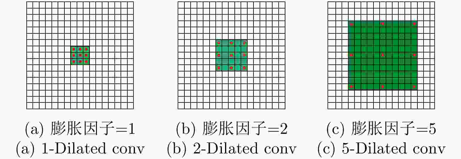
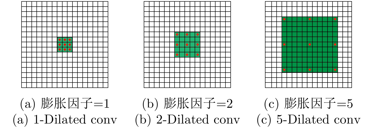
图 1 膨胀卷积原理图

Figure 1. Dilated convolution schematic

下载: 全尺寸图片幻灯片

图 2 残差单元结构

Figure 2. Structure of residual unit

下载: 全尺寸图片幻灯片

图 3 联合感知损失的FRDR-CNN网络结构

Figure 3. Structure of Feature Reuse Dilated-Resnet CNN(FRDR-CNN) with perceptual loss

下载: 全尺寸图片幻灯片

图 4 数据集中的典型场景图

Figure 4. Typical scene graphs in the dataset

下载: 全尺寸图片幻灯片

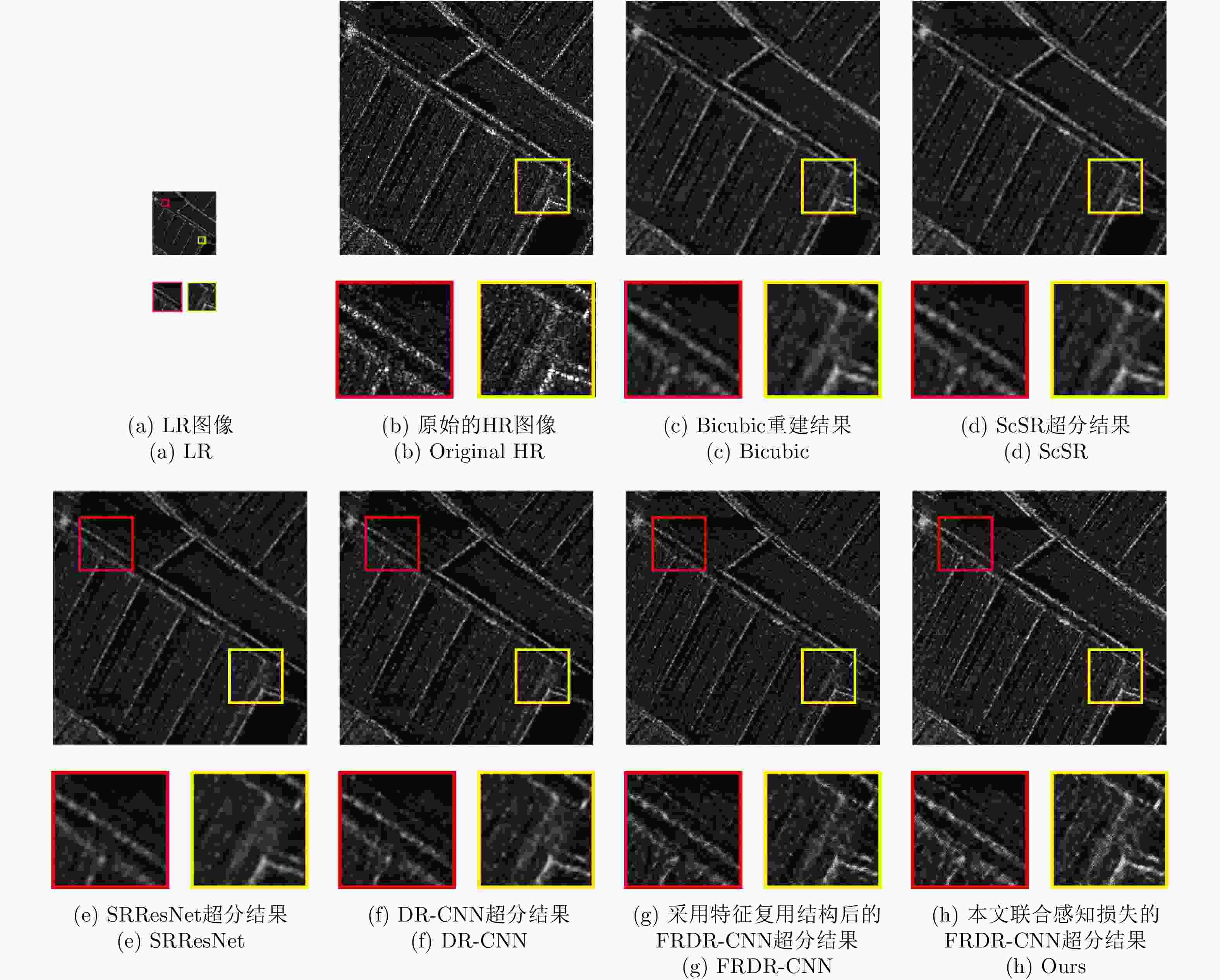
图 5 场景1的SAR图像超分结果及局部放大图

Figure 5. Super resolution results and partial enlargement images of scene 1

下载: 全尺寸图片幻灯片

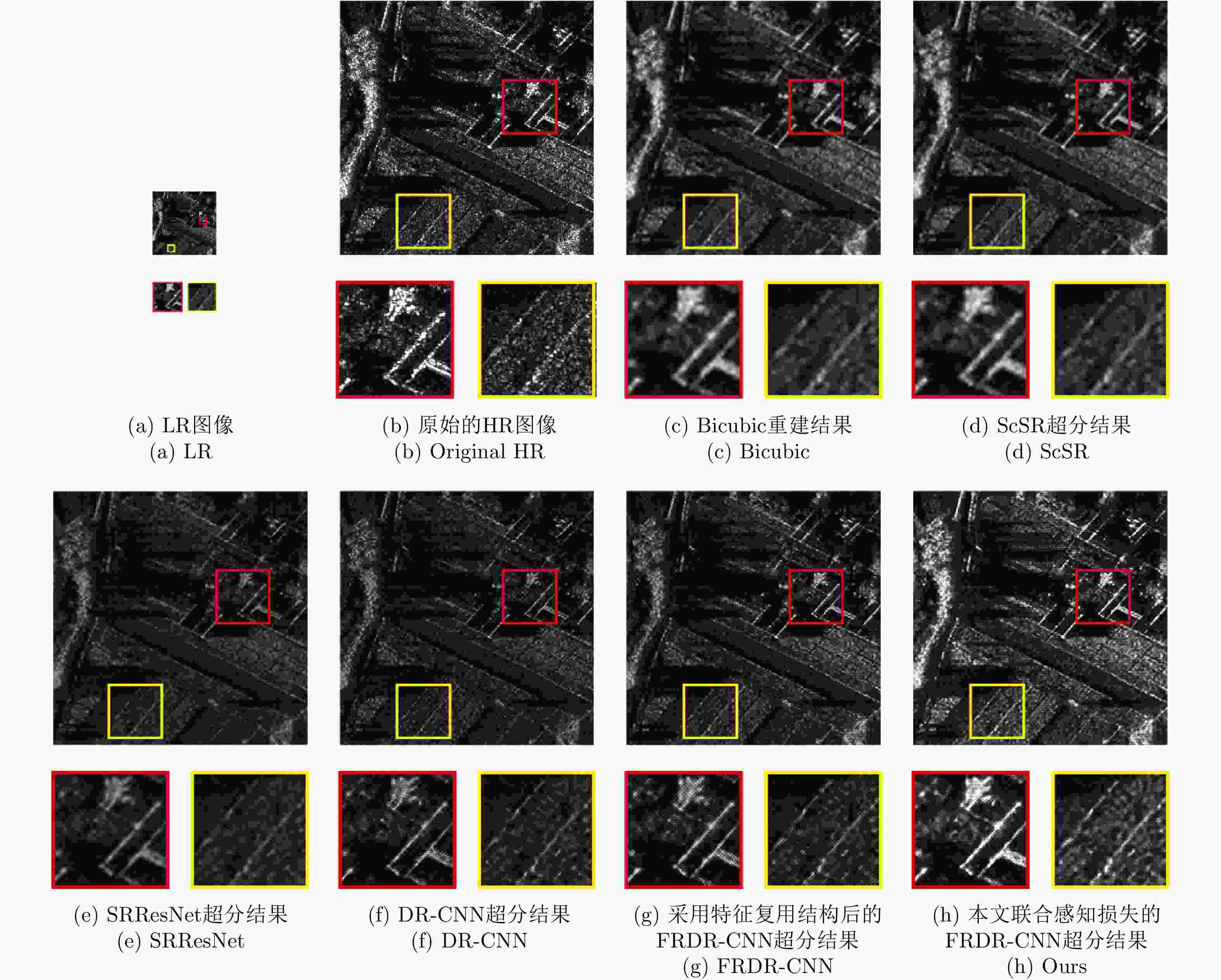
图 6 场景2的SAR图像超分结果及局部放大图

Figure 6. Super resolution results and partial enlargement images of scene 2

下载: 全尺寸图片幻灯片

图 7 5张测试图像的平均SSIM与EPD-ROA值

Figure 7. Average SSIM and EPD-ROA values for five test images

下载: 全尺寸图片幻灯片

表 1 场景1和场景2的SAR图像重建结果表

Table 1. SAR image reconstruction results table of scene 1 and 2

	Results	Bicubic	ScSR	SRResNet	DR-CNN	FRDR-CNN	本文联合感知损失的FRDR-CNN
场景1	PSNR(dB)	29.2897	29.9867	30.4492	30.5922	31.4015	32.4202
	SSIM	0.4755	0.4843	0.4992	0.5023	0.5108	0.5218
	EPD-ROA(HD)	0.3302	0.3773	0.4253	0.4298	0.4329	0.4498
	EPD-ROA(VD)	0.3425	0.3881	0.4378	0.4380	0.4422	0.4556
场景2	PSNR(dB)	29.3572	30.0634	30.6257	31.7901	32.4717	33.4925
	SSIM	0.4532	0.4630	0.4768	0.4796	0.4934	0.5049
	EPD-ROA(HD)	0.3189	0.3596	0.4002	0.4085	0.4142	0.4288
	EPD-ROA(VD)	0.3349	0.3792	0.4198	0.4217	0.4216	0.4352

下载: 导出CSV

参考文献(28)

[1]	BI Zhaoqiang, LI Jian, and LIU Zhengshe. Super resolution SAR imaging via parametric spectral estimation methods[J]. IEEE Transactions on Aerospace and Electronic Systems, 1999, 35(1): 267–281. doi: 10.1109/7.745697
[2]	GUPTA I J, BEALS M J, and MOGHADDAR A. Data extrapolation for high resolution radar imaging[J]. IEEE Transactions on Antennas and Propagation, 1994, 42(11): 1540–1545. doi: 10.1109/8.362783
[3]	BROWN L G. A survey of image registration techniques[J]. ACM Computing Surveys, 1992, 24(4): 325–376. doi: 10.1145/146370.146374
[4]	YANG Siyoung, KIM Y, and JEONG J. Fine edge-preserving technique for display devices[J]. IEEE Transactions on Consumer Electronics, 2008, 54(4): 1761–1769. doi: 10.1109/TCE.2008.4711232
[5]	DUCHON C E. Lanczos filtering in one and two dimensions[J]. Journal of Applied Meteorology, 1979, 18(8): 1016–1022. doi: 10.1175/1520-0450(1979)018<1016:LFIOAT>2.0.CO;2
[6]	YANG Jianchao, WRIGHT J, HUANG T S, et al. Image super-resolution via sparse representation[J]. IEEE Transactions on Image Processing, 2010, 19(11): 2861–2873. doi: 10.1109/TIP.2010.2050625
[7]	DONG Chao, LOY C C, HE Kaiming, et al. Image super-resolution using deep convolutional networks[J]. IEEE Transactions on Pattern Analysis and Machine Intelligence, 2016, 38(2): 295–307. doi: 10.1109/TPAMI.2015.2439281
[8]	KIM J, KWON LEE J, and MU LEE K. Accurate image super-resolution using very deep convolutional networks[C]. The IEEE Conference on Computer Vision and Pattern Recognition, Las Vegas, USA, 2016: 1646–1654. doi: 10.1109/CVPR.2016.182.
[9]	HE Kaiming, ZHANG Xiangyu, REN Shaoqing, et al. Identity mappings in deep residual networks[C]. The 14th European Conference on Computer Vision, Amsterdam, The Netherlands, 2016: 630–645. doi: 10.1007/978-3-319-46493-0_38.
[10]	WANG Longgang, ZHENG Mana, DU Wenbo, et al. Super-resolution SAR image reconstruction via generative adversarial network[C]. 2018 12th International Symposium on Antennas, Propagation and EM Theory, Hangzhou, China, 2018: 1–4.
[11]	LI Zhen, YANG Jinglei, LIU Zheng, et al. Feedback network for image super-resolution[C]. The IEEE/CVF Conference on Computer Vision and Pattern Recognition, Long Beach, USA, 2019: 3862–3871. doi: 10.1109/CVPR.2019.00399.
[12]	KIM J, KWON LEE J, and MU LEE K. Deeply-recursive convolutional network for image super-resolution[C]. The IEEE Conference on Computer Vision and Pattern Recognition, Las Vegas, USA, 2016: 1637–1645. doi: 10.1109/CVPR.2016.181.
[13]	TAI Ying, YANG Jian, and LIU Xiaoming. Image super-resolution via deep recursive residual network[C]. The IEEE Conference on Computer Vision and Pattern Recognition, Honolulu, USA, 2017: 2790–2798. doi: 10.1109/CVPR.2017.298.
[14]	LEDIG C, THEIS L, HUSZÁR F, et al. Photo-realistic single image super-resolution using a generative adversarial network[C]. The IEEE Conference on Computer Vision and Pattern Recognition, Honolulu, USA, 2017: 105–114. doi: 10.1109/CVPR.2017.19.
[15]	YU F and KOLTUN V. Multi-scale context aggregation by dilated convolutions[J]. arXiv preprint arXiv: 1511.07122, 2015.
[16]	HUANG Gao, LIU Zhuang, VAN DER MAATEN L, et al. Densely connected convolutional networks[C]. The IEEE Conference on Computer Vision and Pattern Recognition, Honolulu, USA, 2017: 4700–4708. doi: 10.1109/CVPR.2017.243.
[17]	BENGIO Y, LECUN Y, NOHL C, et al. LeRec: A NN/HMM hybrid for on-line handwriting recognition[J]. Neural Computation, 1995, 7(6): 1289–1303. doi: 10.1162/neco.1995.7.6.1289
[18]	SIMONYAN K and ZISSERMAN A. Very deep convolutional networks for large-scale image recognition[J]. arXiv preprint arXiv: 1409.1556, 2014.
[19]	JOHNSON J, ALAHI A, and LI Feifei. Perceptual losses for real-time style transfer and super-resolution[C]. The 14th European Conference on Computer Vision, Amsterdam, The Netherlands, 2016: 694–711. doi: 10.1007/978-3-319-46475-6_43.
[20]	ZHANG Qiang, YUAN Qiangqiang, LI Jie, et al. Learning a dilated residual network for SAR image despeckling[J]. Remote Sensing, 2018, 10(2): 196. doi: 10.3390/rs10020196
[21]	WANG Panqu, CHEN Pengfei, YUAN Ye, et al. Understanding convolution for semantic segmentation[C]. 2018 IEEE Winter Conference on Applications of Computer Vision, Lake Tahoe, USA, 2018: 1451–1460. doi: 10.1109/WACV.2018.00163.
[22]	SHI Wenzhe, CABALLERO J, HUSZÁR F, et al. Real-time single image and video super-resolution using an efficient sub-pixel convolutional neural network[C]. The IEEE Conference on Computer Vision and Pattern Recognition, Lake Tahoe, USA, 2016: 1874–1883. doi: 10.1109/CVPR.2016.207.
[23]	ZEILER M D, TAYLOR G W, and FERGUS R. Adaptive deconvolutional networks for mid and high level feature learning[C]. 2011 International Conference on Computer Vision, Barcelona, Spain, 2011: 2018–2025. doi: 10.1109/ICCV.2011.6126474.
[24]	NAIR V and HINTON G E. Rectified linear units improve restricted boltzmann machines[C]. The 27th International Conference on Machine Learning, Haifa, Israel, 2010: 807–814.
[25]	王振. 基于学习策略的SAR图像超分辨[D]. [硕士论文], 西安电子科技大学, 2018. WANG Zhen. SAR image super resolution based on learning strategy[D]. [Master dissertation], Xidian University, 2018.
[26]	WANG Qiang and BI Sheng. Prediction of the PSNR quality of decoded images in fractal image coding[J]. Mathematical Problems in Engineering, 2016, 2016: 2159703.
[27]	WANG Zhou, BOVIK A C, SHEIKH H R, et al. Image quality assessment: From error visibility to structural similarity[J]. IEEE Transactions on Image Processing, 2004, 13(4): 600–612. doi: 10.1109/TIP.2003.819861
[28]	唐伶俐, 江平, 戴昌达, 等. 星载SAR图象斑点噪声消除方法效果的比较研究[J]. 环境遥感, 1996, 11(3): 206–211. TANG Lingli, JIANG Ping, DAI Changda, et al. Evaluation of smoothing filters suppressing speckle noise on SAR images[J]. Remote Sensing of Environment China, 1996, 11(3): 206–211.

施引文献

期刊类型引用(4)

1.	葛津津，周浩，凌天庆. 一种应用于脉冲探地雷达前端的探测子系统. 电子测量技术. 2022(04): 27-32 . 百度学术
2.	尹诗，郭伟. 用于探地雷达的超宽带天线设计与仿真. 电子设计工程. 2018(03): 98-102 . 百度学术
3.	宋立伟，张超，洪涛. 冲击波载荷对平面阵列天线电性能的影响. 电子机械工程. 2017(04): 1-5+58 . 百度学术
4.	尹德，叶盛波，刘晋伟，纪奕才，刘小军，方广有. 一种用于高速公路探地雷达的新型时域超宽带TEM喇叭天线. 雷达学报. 2017(06): 611-618 . 本站查看

其他类型引用(6)

资源附件(0)

访问统计

图(7) / 表(1)

计量

文章访问数: 3737
HTML全文浏览量: 1249
PDF下载量: 574
被引次数: 10

1. Introduction
2. Conformal FDA-MIMO Radar
2.1 General conformal FDA-MIMO signal model
2.2 CRLB of conformal FDA-MIMO
3. Reduced-Dimension Target Parameter Estimation Algorithm
4. Simulation Results
4.1 Analysis of computational complexity
4.2 Single target parameter estimation
4.3 Multiple targets parameter estimation
5. Conclusion

1. Introduction
2. Conformal FDA-MIMO Radar
2.1 General conformal FDA-MIMO signal model
2.2 CRLB of conformal FDA-MIMO
3. Reduced-Dimension Target Parameter Estimation Algorithm
4. Simulation Results
4.1 Analysis of computational complexity
4.2 Single target parameter estimation
4.3 Multiple targets parameter estimation
5. Conclusion

参考文献(28)

施引文献

资源附件(0)

访问统计

基于特征复用的膨胀-残差网络的SAR图像超分辨重建

DOI: 10.12000/JR19110

通讯作者:
刘畅 cliu@mail.ie.ac.cn

计量

Super-resolution Reconstruction of SAR Images Based on Feature Reuse Dilated-Residual Convolutional Neural Networks

Corresponding author: LIU Chang, cliu@mail.ie.ac.cn

1. Introduction

2. Conformal FDA-MIMO Radar

2.1 General conformal FDA-MIMO signal model

2.2 CRLB of conformal FDA-MIMO

3. Reduced-Dimension Target Parameter Estimation Algorithm

4. Simulation Results

4.1 Analysis of computational complexity

4.2 Single target parameter estimation

4.3 Multiple targets parameter estimation

5. Conclusion

期刊类型引用(4)

其他类型引用(6)

计量

目录

1. Introduction

2. Conformal FDA-MIMO Radar

2.1 General conformal FDA-MIMO signal model

2.2 CRLB of conformal FDA-MIMO

3. Reduced-Dimension Target Parameter Estimation Algorithm

4. Simulation Results

4.1 Analysis of computational complexity

4.2 Single target parameter estimation

4.3 Multiple targets parameter estimation

5. Conclusion

期刊介绍

联系我们

基于特征复用的膨胀-残差网络的SAR图像超分辨重建

DOI: 10.12000/JR19110

通讯作者: 刘畅 cliu@mail.ie.ac.cn

计量

出版历程

Super-resolution Reconstruction of SAR Images Based on Feature Reuse Dilated-Residual Convolutional Neural Networks

Corresponding author: LIU Chang, cliu@mail.ie.ac.cn

1. Introduction

2. Conformal FDA-MIMO Radar

2.1 General conformal FDA-MIMO signal model

2.2 CRLB of conformal FDA-MIMO

3. Reduced-Dimension Target Parameter Estimation Algorithm

4. Simulation Results

4.1 Analysis of computational complexity

4.2 Single target parameter estimation

4.3 Multiple targets parameter estimation

5. Conclusion

期刊类型引用(4)

其他类型引用(6)

计量

出版历程

目录

1. Introduction

2. Conformal FDA-MIMO Radar

2.1 General conformal FDA-MIMO signal model

2.2 CRLB of conformal FDA-MIMO

3. Reduced-Dimension Target Parameter Estimation Algorithm

4. Simulation Results

4.1 Analysis of computational complexity

4.2 Single target parameter estimation

4.3 Multiple targets parameter estimation

5. Conclusion

期刊介绍

联系我们

通讯作者:
刘畅 cliu@mail.ie.ac.cn