一种极化熵结合混合GEV模型的全极化SAR潮间带区域地物分类方法

折小强; 仇晓兰; 雷斌; 张薇; 卢晓军

doi:10.12000/JR16149

一种极化熵结合混合GEV模型的全极化SAR潮间带区域地物分类方法

DOI: 10.12000/JR16149 CSTR: 32380.14.JR16149

折小强^1,2,3, ,,
仇晓兰^1,2,,
雷斌^1,2,,
张薇^4,,
卢晓军^5,

①.
中国科学院空间信息与应用系统重点实验室北京 100190
②.
中国科学院电子学研究所北京 100190
③.
中国科学院大学北京 100190
④.
民政部卫星减灾应用中心北京 100124
⑤.
中国国际工程咨询公司北京 100048

基金项目: 国家自然科学基金(61331017)，国家高分重大专项(30-Y20A12-9004-15/16)

详细信息

作者简介:
折小强(1989–)，男，陕西绥德人，博士研究生，主要研究方向为极化SAR图像处理。E-mail: sxq@mail.ustc.edu.cn

仇晓兰(1982–)，女，江苏苏州人，中国科学院电子学研究所副研究员，研究方向为SAR成像技术、双基地SAR技术。E-mail: xlqiu@mail.ie.ac.cn

雷　斌(1978–)，男，研究员，研究方向为多传感器遥感信息处理系统体系架构设计、SAR信号并行处理、SAR图像处理与图像质量提升和SAR系统性能预估与优化等。E-mail: leibin@mail.ie.ac.cn

张　薇：女，民政部国家减灾中心。E-mail: zhangwei@ndrcc.gov.cn

卢晓军，江苏泰州人，北京理工大学博士后，中国国际工程咨询公司高级工程师，专业方向为智能控制、信号处理。E-mail: lu8new@163.com

通讯作者:
折小强 sxq@mail.ustc.edu.cn

中图分类号: TN957.52
计量
- 文章访问数: 3214
- HTML全文浏览量: 704
- PDF下载量: 690
- 被引次数: 0
出版历程
- 收稿日期: 2016-12-20
- 修回日期: 2017-02-17
- 网络出版日期: 2017-10-28

A Classification Method Based on Polarimetric Entropy and GEV Mixture Model for Intertidal Area of PolSAR Image

She Xiaoqiang^{1,2,3
, ,},
Qiu Xiaolan^{1,2
,},
Lei Bin^{1,2
,},
Zhang Wei^4
,,
Lu Xiaojun^5
,

①.
Key Laboratory of Technology in Geo-Spatial Information Processing and Application System, Institute of Electronics, Chinese Academy of Sciences, Beijing 100190, China
②.
Institute of Electronics, Chinese Academy of Sciences, Beijing 100190, China
③.
University of Chinese Academy of Sciences, Beijing 100190, China
④.
National Disaster Reduction Center of the Ministry of Civil Affairs, Beijing 100124, China
⑤.
China International Engineering Consulting Corporation, Beijing 100048, China

Funds: The National Natural Science Foundation of China (61331017), The Key Standard Technologies of National High Resolution Special (30-Y20A12-9004-15/16)

摘要

摘要: 该文提出了一种可用于全极化SAR的潮间带区域地物分类的方法。首先针对潮间带的特点对4种典型极化特征进行分析和筛选，得到一组最适合描述潮间带区域的多极化特征：极化熵(Polarimetric entropy)和反熵(Anisotropy)。然后基于对潮间带区域极化熵图像的散射特性分析和极值理论，利用广义极值分布(Generalized Extreme Value, GEV)描述其统计特性。在此基础上，提出了一种基于GEV混合模型的EM算法实现对潮间带地物分类的方法。最后，基于上海崇明东滩潮间带的Radarsat-2全极化数据进行了实验，实验结果证明了方法的有效性。
- 合成孔径雷达(SAR) /
- 多极化特征 /
- 广义极值分布(GEV) /
- 有限混合模型 /
- 潮间带地物分类
Abstract: This paper proposes a classification method for the intertidal area using quad-polarimetric synthetic aperture radar data. In this paper, a systematic comparison of four well-known multipolarization features is provided so that appropriate features can be selected based on the characteristics of the intertidal area. Analysis result shows that the two most powerful multipolarization features are polarimetric entropy and anisotropy. Furthermore, through our detailed analysis of the scattering mechanisms of the polarimetric entropy, the Generalized Extreme Value (GEV) distribution is employed to describe the statistical characteristics of the intertidal area based on the extreme value theory. Consequently, a new classification method is proposed by combining the GEV Mixture Models and the EM algorithm. Finally, experiments are performed on the Radarsat-2 quad-polarization data of the Dongtan intertidal area, Shanghai, to validate our method.
- Synthetic Aperture Radar (SAR) /
- Multi-polarization features /
- Generalized Extreme Value (GEV) distribution /
- Finite Mixture Model (FMM) /
- Intertidal area classification

HTML全文

1. 引言

基于导航卫星的双基地SAR(Bistatic Synthetic Aperture Radar based on Global Navigation Satellite System, GNSS-BSAR)是空-地双基地SAR中一种典型的应用^[1]，使用在轨的导航卫星作为发射源，地面部署接收机(地基、车载、机载)构成双基地SAR系统^[2]。由于导航星座的日趋完善，其全球覆盖性以及重轨特性所带来的优势是其他照射源暂时所不能替代的，其中以地基接收机为主的导航卫星干涉合成孔径雷达(Interference Synthetic Aperture Radar based on the Global Navigation Satellite System, GNSS-InSAR)在场景形变监测领域有着广阔的应用前景^[3]，成为了近年来研究热点。

在GNSS-BSAR系统成像方面，已有研究者分别使用不同的导航卫星星座进行了成像验证，包括了北斗^[4,5]、GPS^[6]、格洛纳斯^[7]、伽利略^[8]。除此以外文献[9]还提出了多角度融合方法以增强图像信噪比。在形变监测方面，来自伯明翰大学的学者们^[10]使用直达波天线，配合长约50 m的线缆构建了理想点目标，并使用格洛纳斯作为发射源，首次实现了精度约为1 cm的1维形变反演结果。该实验初步验证了GNSS-InSAR应用于形变监测的可行性。为了进一步验证场景形变监测的可能，2017年文献[11]通过对接收机进行高精度移位来模拟场景建筑形变，成功反演出了形变，精度约为1 cm。在3维形变方面，2018年北京理工大学的技术团队^[12]通过人为构建转发器，进行了精度可控的强点目标形变模拟，使用我国的北斗IGSO卫星，成功实现了精度优于5 mm的3维形变反演，这些验证性实验充分表明了GNSS-InSAR应用于场景形变检测的可能。

若要实现GNSS-InSAR场景的3维形变反演，需要同时至少3颗卫星从不同角度照射场景。由于GNSS-InSAR系统的拓扑高度非对称性以及导航信号的窄带特性^[13]，加上导航卫星的重轨并非是严格意义上的重轨，除了不可避免的空间基线外，重轨时间也并非严格一致，因此在实际数据采集中，需要对系统构型以及数据采集时间进行严格的优化设计。文献[14]提出了一种联合优化方法，解决了面向大场景下的多星多角度构型优化问题，配合多个接收机实现综合分辨性能优异的大场景成像。文献[15]提出了空间去相干的理论描述框架，表明了空间去相干在GNSS-InSAR中的必要性，但未对数据采集时间进行说明。从当前实际情况出发，不精确的数据采集时间可能会造成存储资源浪费，空间去相干导致的数据截取进一步降低了数据有效性。具体如图1所示：

图 1 数据截取与有效数据示意图

Figure 1. Effective data interception diagram

下载: 全尺寸图片幻灯片

针对上述问题，本文提出了一种GNSS-InSAR场景连续数据采集优化方法，通过结合当前数据的卫星轨迹和两行星历数据文件(STK Two-Line Element sets, TLE)预测轨迹，基于相干系数轨迹对齐，获取卫星重轨时间间隔，得到最优的数据采集策略，从源头上降低数据的空间去相干性，提升所采集数据有效性，节约存储资源。在第2部分对GNSS-InSAR场景数据采集优化方法进行了详细介绍。第3部分针对提出的方法进行了实验设计，开展了实测数据采集，并针对采集的数据进行了初步分析。第4部分对全文进行总结。

2. GNSS-InSAR场景数据采集优化模型

2.1 GNSS-InSAR相干系数理论模型

对于GNSS-InSAR图像而言，经过保相成像处理后，场景中任意一点 $\left( {{x_0},{y_0}} \right)$ 的像素信息分别对应分辨单元内所有散射体回波的相参叠加，可建模为

$\begin{aligned} s\left( {{x_0},{y_0}} \right) =& \iint f\left( {x,y;t} \right){\rm{exp}}\left[ {{\rm{ - j}}\frac{{2{\rm{\pi}} }}{\lambda }r\left( {x,y;{ P}} \right)} \right]\\ & \cdot {W}\left( {{x - }{{x}_0}{,y - }{{y}_0};{ P}} \right){\rm{d}}{x}{\rm{d}}{y} +{n}\left( {{{x}_0},{{y}_0};{t}} \right)\\ \end{aligned}$

(1)

其中， ${f}\left( {{x},{y};{t}} \right)$ 为时间 $t$ 下的地表散射系数， ${{P}}$ 为对应的合成孔径中心位置矢量， ${W}\left( {{x},{y};{ P}} \right)$ 表示系统的点扩散函数(PSF), ${n}\left( {{x},{y};{t}} \right)$ 为图像的加性噪声。对于SAR图像的同名点像素，其相干系数可表示为^[16]

$\rho =\frac{{\displaystyle\iint {{{s}_{\rm{m}}}\left( {{{x}_0},{{y}_0}} \right){s}_{\rm{s}}^{\rm{*}}\left( {{{x}_0},{{y}_0}} \right){\rm{d}}{x}{\rm{d}}{y}}}}{{\sqrt {\displaystyle\iint {{{s}_{\rm{m}}}\left( {{{x}_0},{{y}_0}} \right){s}_{\rm{m}}^{\rm{*}}\left( {{{x}_0},{{y}_0}} \right){\rm{d}}{x}{\rm{d}}{y}}\displaystyle\iint {{{s}_{\rm{s}}}\left( {{{x}_0},{{y}_0}} \right){s}_{\rm{s}}^{\rm{*}}\left( {{{x}_0},{{y}_0}} \right){\rm{d}}{x}{\rm{d}}{y}}} }}$

(2)

其中，下标m表示主图像， ${\rm{s}}$ 表示辅图像。根据柯西不等式可以判断： $0 \le \rho \le 1$ ，当 $\rho = 0$ 时表示同名点完全不相干，当 $\rho = 1$ 时，同名点完全相干。

将点目标像素模型式(1)带入到式(2)并化简得到

$\rho =\frac{\displaystyle\iint{{{s}_{{\rm av}}}\left( x,y \right){\rm exp}\left[ -{\rm j}\frac{2{\rm{\pi}} }{\lambda }\bigr( r\left( x,y;{{{P}}_{{\rm m}}} \bigr)-r\left( x,y;{{{P}}_{{\rm s}}} \right) \right) \right]}{{\Bigr| W\left( x-{{x}_{0}},y-{{y}_{0}};{{{P}}_{{\rm m}}} \right) \Bigr|}^{2}}{\rm d}x{\rm d}y}{\sqrt{\begin{array}{l} \left( \displaystyle\iint{{{s}_{{\rm m}}}\left( x,y \right){\rm exp}\left[ -{\rm j}\frac{2{\rm{\pi}} }{\lambda }r\left( x,y;{{{{P}}}_{{\rm m}}} \right) \right]}{{\Bigr| W\left( x-{{x}_{0}},y-{{y}_{0}};{{{P}}_{{\rm m}}} \right) \Bigr|}^{2}}{\rm d}x{\rm d}y+{{n}_{{\rm m}}} \right) \\ \times\left( \displaystyle\iint{{{s}_{{\rm s}}}\left( x,y \right){\rm exp}\left[ {\rm +j}\frac{2{\rm{\pi}} }{\lambda }r\left( x,y;{{{P}}_{{\rm s}}} \right) \right]}{{\Bigr| W\left( x-{{x}_{0}},y-{{y}_{0}};{{{P}}_{{\rm m}}} \right) \Bigr|}^{2}}{\rm d}x{\rm d}y+{{n}_{{\rm s}}} \right) \end{array}}}$

(3)

式(3)的推导使用了如下近似：

(1) 由于导航卫星的高轨道特性，使得 ${W}\left( {x - }{{x}_0},\right.$ $\left.{{y - }{{y}_0};{{ P}_{\rm{m}}}} \right) \approx {W}\left( {{x - }{{x}_0},{y - }{{y}_0};{{ P}_{\rm{s}}}} \right)$ 成立；

(2) 相邻两天的噪声相干系数为0，即

${n}\left( {{{x}_0},{{y}_0};{{t}_{\rm{m}}}} \right) \times {n}\left( {{{x}_0},{{y}_0};{{t}_{\rm{s}}}} \right) = 0$

(4)

(3) 相邻两天的目标散射系数为 ${{s}_{{\rm{av}}}}\left( {{x},{y}} \right)$ ，即

${{s}_{{\rm{av}}}}\left( {{x},{y}} \right) \approx {f}\left( {{x},{y};{{t}_{\rm{m}}}} \right){{f}^{\rm{*}}}\left( {{x},{y};{{t}_{\rm{s}}}} \right)$

(5)

对式(3)中的相干系数 $\rho$ 进一步分解得到

$\rho = {\rho _{{\rm{th}}}} \times {\rho _{{\rm{ti}}}} \times {\rho _{{\rm{sp}}}}$

(6)

其中，热噪声相干系数 ${\rho _{{\rm{th}}}}$ 与时间相干系数 ${\rho _{{\rm{ti}}}}$ 分别由系统与实际目标决定。

对于PS点^[17]而言，地表散射系数相对稳定，不随时间变化，同时为了便于后续分析，假定散射系数为1得到空间相干系数 ${\rho _{{\rm{sp}}}}$ 的简化式为

${\rho _{{\rm{sp}}}} = \frac{{\displaystyle\iint {{\rm{exp}}\left[ {{ - }{\rm{j}}\dfrac{{2{\rm{\pi}} }}{\lambda }\bigr( {{r}\left( {{x},{y};{{ P}_{\rm{m}}}} \right){ - r}\left( {{x},{y};{{ P}_{\rm{s}}}} \right)} \bigr)} \right]{{\Bigr| {{W(x - }{{x}_0},{y - }{{y}_0};{{ P}_{\rm{m}}}{)}} \Bigr|}^2}{\rm{d}}{x}{\rm{d}}{y}}}}{{\sqrt {\left( {\displaystyle\iint {{{\Bigr| {{W}\left( {{x - }{{x}_0},{y - }{{y}_0};{{ P}_{\rm{m}}}} \right)} \Bigr|}^2}{\rm{d}}{x}{\rm{d}}{y}}} \right)\left( {\displaystyle\iint {{{\Bigr| {{W(x - }{{x}_0},{y - }{{y}_0};{{ P}_{\rm{m}}}{)}} \Bigr|}^2}{\rm{d}}{x}{\rm{d}}{y}}} \right)} }}$

(7)

从式(7)推导结果可以知道，空间基线主要是影响 ${r}\left( {{x},{y};{ P}} \right)$ 从而导致空间去相干。

2.2 数据采集优化模型

导航卫星的重轨时间并非稳定不变，因此需要对数据采集时间进行有效预测，从源头上降低空间去相干，提高数据有效性。

假定主图像数据采集时间为 ${{t}_{\rm{m}}}$ ，该采集时间可以通过文献[14]中的广义优化模型进行求解，辅图像数据采集时间为 ${{t}_{\rm{s}}}={{t}_{\rm{m}}}+\Delta {t}$ , $\Delta t$ 为时间间隔，那么最优化数据采集模型可通过式(7)推导而来

$\begin{split} \Delta {t }=&{\rm{arg}}\;{\rm{max}}\left\{ \iint {{\left| {{\widetilde W}\left( {{x},{y};{{ P}_{\rm{m}}}} \right)} \right|}^2} {\rm{exp}}\left[ {{ - }{\rm{j}}\frac{{2{\rm{\pi}} }}{\lambda }\bigr( {{r}\left( {{x},{y};{{ P}_{\rm{m}}}} \right){ - r}\left( {{x},{y};{ P}\left( {{{t}_{\rm{m}}}+\Delta {t}} \right)} \right)} \bigr)} \right] {\rm{d}}{x}{\rm{d}}{y} \right\} \end{split}$

(8)

其中， ${\widetilde W}\left( {{x},{y};{{ P}_{\rm{m}}}} \right)$ 为 ${t_{\rm{m}}}$ 下等效归一化PSF, ${ P}\left( {{{t}_{\rm{m}}} +}\right.$ $\left.\Delta {t} \right)$ 为 $\Delta {t}$ 时间偏置下得合成孔径中心位置矢量。

第1天数据采集需要进行实验设计以确定最优数据采集时刻，往后的重轨天数据采集可以根据数据采集优化模型，同时结合星历文件进行预测。整体的预测流程如图2所示， ${n}$ 为任意一天采集的数据， ${k}$ 为重轨天数间隔。

图 2 GNSS-InSAR数据采集时间优化流程

Figure 2. Time optimization process of GNSS-InSAR data acquisition

下载: 全尺寸图片幻灯片

实际卫星位置对应的实际时间设为 ${{t}_{n}}$ ，经过模型优化得到的时间偏差为 $\Delta {t}$ ，那么第 ${n} + {k}$ 天对应的实际数据采集时间可表示为

${{t}_{{n}+{k}}} = {{t}_{n}} + \Delta {t}$

(9)

3. 实验验证

3.1 GNSS-InSAR场景3维形变反演实验设计

对于固定场景的形变监测，首次数据采集的时候需要严格设计系统构型，使分辨率达到最优化。本次实验接收机部署在北京理工大学信息科学试验楼楼顶西北角，实施监测场景位于西偏北30°。使用理论分辨率计算公式^[18]对该场景进行分辨率设计。仿真参数具体参见表1。

表 1 数据采集试验仿真参数

Table 1. Data acquisition test simulation parameters

参数	值
照射源	北斗 IGSO1～5
PRF	1000 Hz
带宽	10.23 MHz
合成孔径时间	600 s
TLE文件更新日期	2019年4月29日
预定数据采集日期	2019年4月30日

下载: 导出CSV

| 显示表格

以分辨单元面积作为判定依据，得到预定采集日期当天全时段下各个卫星在预定场景下所能得到的分辨单元面积如图3所示。

图 3 全时段下场景分辨单元面积

Figure 3. Scene resolution unit area in full time

下载: 全尺寸图片幻灯片

为了实现3维形变反演，需要同一时间下有3颗卫星对场景进行照射。图3中10点前后与17点前后满足当前场景上空有3颗IGSO卫星可见的条件。更进一步，为了使分辨单元面积达到最优，可以得到具体的数据采集时间。具体如图4红框标注，分别是9点30分前后与17点30分前后。

图 4 首次数据采集时间设计结果

Figure 4. Design results of first data acquisition time

下载: 全尺寸图片幻灯片

为了配合实验，在场景布置转发器，整体的系统构型如图5所示。

图 5 GNSS-InSAR场景3维形变反演实验拓扑构型设计结果

Figure 5. GNSS-InSAR topological configuration design results of 3D deformation retrieval experiment

下载: 全尺寸图片幻灯片

3.2 重轨数据采集时间优化

以2019年4月30日采集的实测数据作为第 ${n}$ 天数据，对于北斗的IGSO而言，重轨时间约为1天，即 ${m}$ =1，同时下载当天最新的TLE文件。以IGSO1为例，结合图2进行详细说明：

(1) 使用实测数据的直达波进行卫星位置解算，同时根据TLE文件推算当天和相邻天的卫星轨迹。经过相干系数轨迹匹配之后，得到的轨迹如图6所示。

图 6 对齐后的TLE卫星轨迹与实测数据卫星轨迹

Figure 6. Aligned TLE satellite trajectory and measured data satellite trajectory

下载: 全尺寸图片幻灯片

(2) 以匹配得到的TLE卫星轨迹作为参考，对重轨天的TLE卫星轨迹进行数据采集优化模型求解，系统的PSF与优化模型仿真结果分别如图7与图8所示。

图 7 场景[–147, 20, 0]处理论PSF

Figure 7. Theoretical PSF in scene at position of [–147, 20, 0]

下载: 全尺寸图片幻灯片

图 8 数据采集优化模型仿真结果

Figure 8. Simulation results of data acquisition optimization model

下载: 全尺寸图片幻灯片

对图8的结果分析可知，第1个峰值点为其本身，由于空间基线为0，相干系数为1。第2个峰值点相干系数为0.999644，满足除了第1个峰值点外相邻天相干系数最大值条件，因此第2个峰值点就是最佳重轨时的空间相干系数。此时经过模型优化得到的时间间隔为： $\Delta t = 86163\;{\rm{s}} = 23\;{\rm{h}}\;56\;\min 3\;{\rm{s}}$ ，结合第1天的实测数据轨迹对应的时间 ${t_1} = 9\;{\rm{h}}\;26\;\min \;0\;{\rm{s}}$ ，第2天准确的数据采集时间为： ${t_2} = 9\;{\rm{h}}\;22\;\min 3\;{\rm{s}}$ 。

3.3 结果分析

为了说明优化结果的正确性，在实验场景中放置转发器模拟理想点目标(图5)，同时按照优化后的时间进行5月1日数据采集。实际采集时间为 $9\;{\rm{h}}\;21\;\min \;53\;{\rm{s}}$ ，总采集时间约650 s。相邻两天的空间相干系数轨迹匹配结果如图9所示。

图 9 实测数据重轨空间相干系数

Figure 9. The spatial coherence coefficient of measured data

下载: 全尺寸图片幻灯片

从图9中峰值点位置来看，重轨数据采集优化模型得到的结果和实际结果相吻合。为了进一步说明，图10给出了IGSO1卫星实测数据成像结果。

图 10 场景成像结果

Figure 10. Imaging results of scene

下载: 全尺寸图片幻灯片

对相邻两天的图像相干系数进行求解，得到图11所示结果。在同一坐标系下，仿真目标位于[–147, 20, 0]，空间相干系数为0.999644；转发器位于[–147, 20, 0]，相干系数为0.9996；两者的相干系数基本保持一致。

图 11 相干系数结果

Figure 11. Coherence coefficient result

下载: 全尺寸图片幻灯片

图9与图10的结果表明经过数据采集优化模型后得到的时间间隔与实际卫星轨迹的重轨时间相互吻合，在保证600 s预期合成孔径时间下，可以最大限度减少数据采集时间，节约存储资源。同时避免后期由于数据对齐带来的数据有效性降低问题。

4. 结论

在GNSS-InSAR场景1维/3维形变反演应用中，针对由于导航卫星重轨时间的非严格一致性与有效数据截取带来的数据冗余，数据有效性低等问题，本文提出了一种面向GNSS-InSAR场景数据采集的优化模型，采用实测数据与TLE文件相结合，根据当天数据采集时间，预测相邻天重轨时间，从而实现精确的数据采集。实测数据验证结果表明了数据采集时间优化模型的正确性。该方法的提出有利于GNSS-InSAR场景1维/3维形变反演实验的开展，在降低原始数据冗余度基础上，保证了有效数据时间长度大于预期合成孔径时间。

图 1 潮间带的极化特征示例

Figure 1. Examples of multi-polarization features of intertidal area

下载: 全尺寸图片幻灯片

图 2 GEV分布的3种形态

Figure 2. Three types of the GEV distribution

下载: 全尺寸图片幻灯片

图 3 基于GEVMM的图像分类流程

Figure 3. Flowchart of GEVMM

下载: 全尺寸图片幻灯片

图 4 所选实验区域

Figure 4. The selected study area

下载: 全尺寸图片幻灯片

图 5 研究区域的极化特征

Figure 5. Multi-polarization features of the study area

下载: 全尺寸图片幻灯片

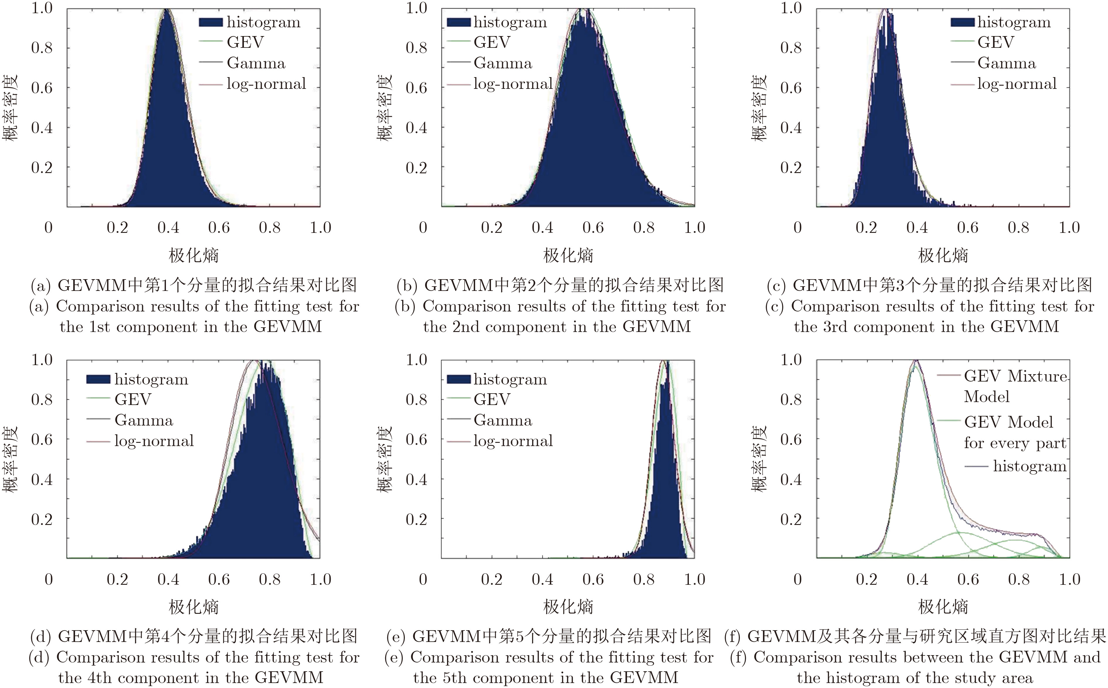
图 6 GEVMM及其各分量与Gamma分布和log-normal分布的对比：(a)–(e)分别为5个分量与Gamma分布，log-normal分布以及对应标记区域的直方图的对比，其中蓝色区域为归一化直方图，绿线是GEV拟合结果，黑线是Gamma拟合结果，红线是log-normal拟合结果，(f)给出了GEVMM及其各个分量与研究区域直方图的对比结果，其中蓝线为归一化直方图，红线为GEVMM，绿线为GEVMM的各个分量

Figure 6. Fitness comparison among GEV distribution and Gamma distribution and Log-normal distribution of each component in GEVMM: (a)–(e) represent the five components of the GEVMM and the fitting results by the Gamma distribution and log-normal distribution for the histograms, which are marked as blue, the green lines represent the GEV fitting results, the black lines represent the most fitted Gamma distribution and the red lines represent the most fitted log-normal distribution, (f) shows the five components of GEVMN as green lines and the respective histograms as blue lines, the red line represents the final model

下载: 全尺寸图片幻灯片

图 7 潮间带的地物分类实验结果

Figure 7. Classification results of the intertidal area

下载: 全尺寸图片幻灯片

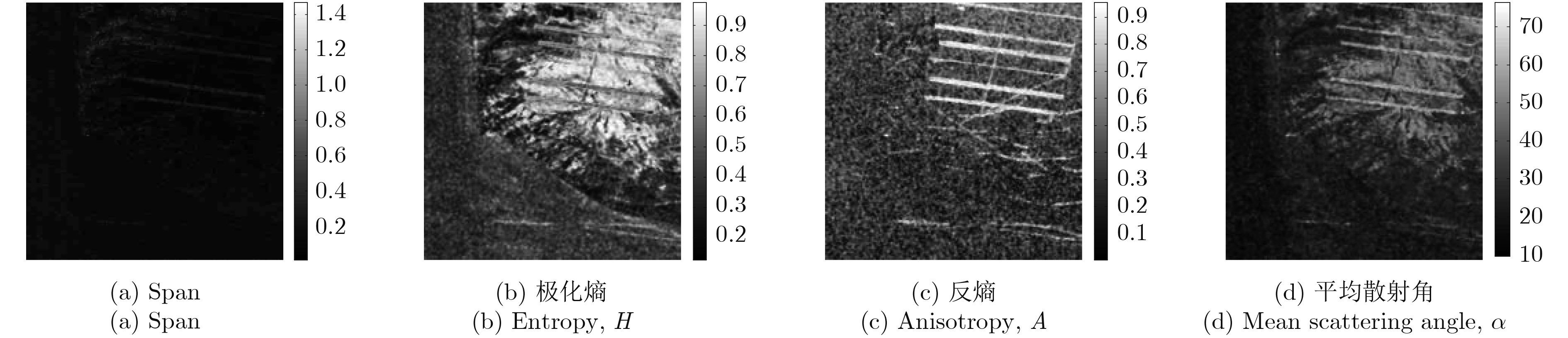
表 1 各极化特征的Michelson类间对比度

Table 1. Michelson between-region contrast of different features

极化特征	类间对比度
Span	0.4092
Entropy	0.7703
Anisotropy	0.9959
α	0.6757

下载: 导出CSV

表 2 GEV分布，Gamma分布和log-normal分布在每种类别中的拟合结果的AIC值

Table 2. The AIC values of the fitting results between the GEV distribution, the Gamma distribution and log-normal distribution

AIC	1	2	3	4	5
GEV	6.3988	4.0095	4.1105	4.7009	6.2093
Gamma	11.3878	9.3573	7.6928	9.0210	8.3989
log-normal	11.3878	9.3573	7.6928	9.0213	8.3997

下载: 导出CSV

参考文献(32)

[1]	Lee Hoonyol, Chae Heesam, and Cho Seong-Jun. Radar backscattering of intertidal mudflats observed by Radarsat-1 SAR images and ground-based scatterometer experiments[J]. IEEE Transactions on Geoscience and Remote Sensing, 2011, 49(5): 1701–1711. doi: 10.1109/TGRS.2010.2084094
[2]	Li Xiaofeng, Li Chunyan, Xu Qing, et al.. Sea surface manifestation of along-tidal-channel underwater ridges imaged by SAR[J]. IEEE Transactions on Geoscience and Remote Sensing, 2009, 47(8): 2467–2477. doi: 10.1109/TGRS.2009.2014154
[3]	Won Eun-Sung, Ouchi Kazuo, and Yang Chan-Su. Extraction of underwater laver cultivation nets by SAR polarimetric entropy[J]. IEEE Geoscience and Remote Sensing Letters, 2013, 10(2): 231–235. doi: 10.1109/LGRS.2012.2199077
[4]	Inglada J and Garello R. Underwater bottom topography estimation from SAR images by regulariziation of the inverse imaging mechanism[C]. IEEE 2000 International Geoscience and Remote Sensing Symposium, 2000, 5: 1848–1850.
[5]	Kim Ji-Eun, Park Sang-Eun, Kim Duk-Jin, et al.. Recent advances in POL(in)SAR remote sensing & stress-change monitoring of wetlands with applications to the Sunchon Bay Tidal Flats[C]. Synthetic Aperture Radar European Conference (EUSAR), Friedrichshafen, Germany, 2008: 1–3.
[6]	Park S E, Moon W M, and Kim D J. Estimation of surface roughness parameter in intertidal mudflat using airborne polarimetric SAR data[J]. IEEE Transactions on Geoscience and Remote Sensing, 2009, 47(4): 1022–1031.
[7]	Zhen Li, Heygster G, and Notholt J. Intertidal topographic maps and morphological changes in the German Wadden Sea between 1996–1999 and 2006–2009 from the Waterline method and SAR images[J]. IEEE Journal of Selected Topics in Applied Earth Observations & Remote Sensing, 2014, 7(8): 3210–3224.
[8]	Kim Duk-Jin, Park Sang-Eun, Lee Hyo-Sung, et al.. Investigation of multiple frequency polarimetric SAR signal backscattering from tidal flats[C]. International Geoscience and Remote Sensing Symposium, 2009: 896–899.
[9]	Sine Skrunes, Camilla Brekke, and Torbjorn Eltoft. Characterization of marine surface slicks by Radarsat-2 multi-polarization features[J]. IEEE Transactions on Geoscience and Remote Sensing, 2014, 52(9): 5302–5319. doi: 10.1109/TGRS.2013.2287916
[10]	Cloude S R and Pottier E. A review of target decomposition theorems in radar polarimetry[J]. IEEE Transactions on Geoscience and Remote Sensing, 1996, 34(2): 498–518. doi: 10.1109/36.485127
[11]	邢艳肖, 张毅, 李宁, 等. 一种联合特征值信息的全极化SAR图像监督分类方法[J]. 雷达学报, 2016, 5(2): 217–227. doi: 10.12000/JR16019 Xing Yanxiao, Zhang Yi, Li Ning, et al.. Polarimetric SAR image supervised classification method integrating eigenvalues[J]. Journal of Radars, 2016, 5(2): 217–227. doi: 10.12000/JR16019
[12]	孙勋, 黄平平, 涂尚坦, 等. 利用多特征融合和集成学习的极化SAR图像分类[J]. 雷达学报, 2016, 5(6): 692–700. doi: 10.12000/JR15132 Sun Xun, Huang Pingping, Tu Shangtan, et al.. Polarimetric SAR image classification using multiple-feature fusion and ensemble learning[J]. Journal of Radars, 2016, 5(6): 692–700. doi: 10.12000/JR15132
[13]	邵璐熠, 洪文. 基于二维极化特征的POLSAR图像决策分类[J]. 雷达学报, 2016, 5(6): 681–691. doi: 10.12000/JR16002 Shao Luyi and Hong Wen. Dicision tree classification of POLSAR image based on two-dimensional polarimetric features[J]. Journal of Radars, 2016, 5(6): 681–691. doi: 10.12000/JR16002
[14]	Fukuda S. Relating polarimetric SAR image texture to the scattering entropy[C]. IEEE International Geoscience and Remote Sensing Symposium, 2004: 2475–2478.
[15]	Cloude S R and Papathanassiou K P. Surface roughness and polarimetric entropy[C]. IEEE 1999 International Geoscience and Remote Sensing Symposium, 1999: 2443–2445.
[16]	Cloude S R and Pottier E. An entropy based classification scheme for land applications of polarimetric SAR[J]. IEEE Transactions on Geoscience and Remote Sensing, 1997, 35(1): 68–78. doi: 10.1109/36.551935
[17]	Won E S and Ouchi K. A novel method to estimate underwater marine cultivation area by using SAR polarimetric entropy[C]. 2011 IEEE International Geoscience and Remote Sensing Symposium, 2011: 2097–2100.
[18]	滑文强, 王爽, 侯彪. 基于半监督学习的SVM-Wishart极化SAR图像分类方法[J]. 雷达学报, 2015, 4(1): 93–98. doi: 10.12000/JR14138 Hua Wen-qiang, Wang Shuang, and Hou Biao. Semi-supervised Learning for Classifcation of polarimetric SAR images based on SVM-Wishart[J]. Journal of Radars, 2015, 4(1): 93–98. doi: 10.12000/JR14138
[19]	Doulgeris A P, Akbari V, and Eltoft T. Automatic PolSAR segmentation with the u-distribution and Markov random fields[C]. The 9th European Conference on Synthetic Aperture Radar, 2012: 183–186.
[20]	Li Zhen, Heygester Georg, and Notholt J. The topography comparsion between the year 1999 and 2006 of German tidal flat wadden sea analyzing SAR images with waterline method[C]. 2013 IEEE International Geoscience and Remote Sensing Symposium, 2013: 2443–2446.
[21]	Li Zhen, Heygester G, and Notholt J. Topographic mapping of Wadden Sea with SAR images and waterlevel model data[C]. IEEE International Geoscience and Remote Sensing Symposium, 2012: 2645–2648.
[22]	Li Zhen, Heygester Georg, and Notholt J. Topographic mapping of Wadden Sea, with SAR images and waterlevel model data[C]. 2012 IEEE International Geoscience and Remote Sensing Symposium, 2012: 2645–2648.
[23]	Wal D V D, Herman P M J, and Dool W V D. Characterisation of surface roughness and sediment texture of intertidal flats using ERS SAR imagery[J]. Remote Sensing of Environment, 2005, 98(1): 96–109. doi: 10.1016/j.rse.2005.06.004
[24]	Geng X M, Li X M, Velotto D, et al.. Study of the polarimetric characteristics of mud flats in an intertidal zone using C-and X-band spaceborne SAR data[J]. Remote Sensing of Environment, 2016, 176: 56–68. doi: 10.1016/j.rse.2016.01.009
[25]	Ding Hao, Huang Yong, and Liu Ningbo. Modeling of sea spike events with generalized extreme value distribution[C]. 2015 European Radar Conference, 2015: 113–116.
[26]	李恒超. 合成孔径雷达图像统计特性分析及滤波算法研究[D]. [博士论文], 中国科学院电子学研究所, 2007. Li Heng-chao. Research on statistical analysis and despeckling algorithm of synthetic aperture radar images[D]. [Ph.D. dissertation], Institute of Electronics, Chinese Academy of Sciences, 2007.
[27]	Embrechts P. Quantitative Risk Management[M]. Quantitative Risk Management, Princeton University Press, 2005: 67–73.
[28]	熊太松. 基于统计混合模型的图像分割方法研究[D]. [博士论文], 电子科技大学, 2013. Xiong Taisong. The study of image segmentation based on statistical mixture models[D]. [Ph.D. dissertation], University of Electronic Science and Technology of China, 2013.
[29]	Prescott P and Walden A T. Maximum iikelihood estimation of the parameters of the generalized extreme-value distribution[J]. Biometrika, 1980, 67(3): 723–724. doi: 10.1093/biomet/67.3.723
[30]	Peli E. Contrast in complex images[J]. Journal of the Optical Society of America A, 1990, 7(10): 2032–2040. doi: 10.1364/JOSAA.7.002032
[31]	Sine Skrunes, Camilla Brekke, and Torbjorn Eltoft. Characterization of marine surface slicks by Radarsat-2 multipolarization features[J]. IEEE Transactions on Geoscience and Remote Sensing, 2014, 52(9): 5302–5319. doi: 10.1109/TGRS.2013.2287916
[32]	Akaike H. Information theory and an extension of the maximum likelihood principle[C]. 2nd International Symposium on Information Theory, Budapest, 1973: 267–281.

施引文献

资源附件(0)

访问统计

图(7) / 表(2)

计量

文章访问数: 3214
HTML全文浏览量: 704
PDF下载量: 690
被引次数: 0

1. 引言
2. GNSS-InSAR场景数据采集优化模型
2.1 GNSS-InSAR相干系数理论模型
2.2 数据采集优化模型
3. 实验验证
3.1 GNSS-InSAR场景3维形变反演实验设计
3.2 重轨数据采集时间优化
3.3 结果分析
4. 结论

一种极化熵结合混合GEV模型的全极化SAR潮间带区域地物分类方法

DOI: 10.12000/JR16149 CSTR: 32380.14.JR16149

通讯作者:
折小强 sxq@mail.ustc.edu.cn

计量