
 Submit Manuscript
 Peer Review
 Editor Work
- Home
- Articles & Issues
-
Data
- Dataset of Radar Detecting Sea
- SAR Dataset
- SARGroundObjectsTypes
- SARMV3D
- AIRSAT Constellation SAR Land Cover Classification Dataset
- 3DRIED
- UWB-HA4D
- LLS-LFMCWR
- FAIR-CSAR
- MSAR
- SDD-SAR
- FUSAR
- SpaceborneSAR3Dimaging
- Sea-land Segmentation
- SAR Multi-domain Ship Detection Dataset
- SAR-Airport
- Hilly and mountainous farmland time-series SAR and ground quadrat dataset
- SAR images for interference detection and suppression
- HP-SAR Evaluation & Analytical Dataset
- GDHuiYan-ATRNet
- Multi-System Maritime Low Observable Target Dataset
- DatasetinthePaper
- DatasetintheCompetition
- Report
- Course
- About
- Publish
- Editorial Board
- Chinese
| Citation: | WANG Jingjing, LIU Zheng, XIE Rong, et al. HRRP target recognition method for full polarimetric radars by combining Cameron decomposition and fusing RKELM[J]. Journal of Radars, 2021, 10(6): 944–955. doi: 10.12000/JR21099

|
HRRP Target Recognition Method for Full Polarimetric Radars by Combining Cameron Decomposition and Fusing RKELM
DOI: 10.12000/JR21099 CSTR: 32380.14.JR21099
More Information-
Abstract
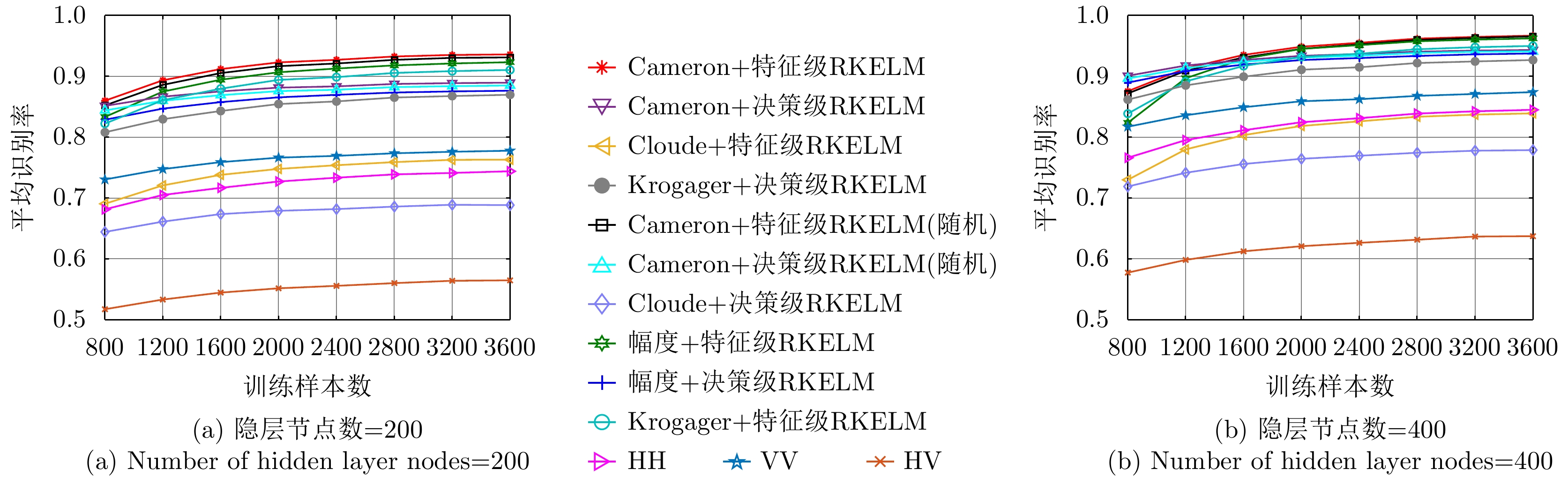
A recognition method combining Cameron decomposition and fusing Reduced Kernel Extreme Learning Machine (RKELM) is proposed for the Full Polarimetric (FP) High Resolution Range Profile (HRRP)-based radar target recognition task. In the feature extraction phase, Cameron decomposition is exploited to define the projection component of the target on the standard scatterers. Through analysis, the projection components on three scattering bases, i.e., trihedral, dihedral, and 1/4 wave device, are selected as target features, which achieve more detailed descriptions of the target characteristics. In the classification phase, considering the instability of the recognition performance of the RKELM algorithm, the RKELM based on prototype clustering preprocessing is first proposed. Then, to improve the recognition performance, we proposed the feature level fusing RKELM and the decision level fusing RKELM to fuse the three projection components of the targets. The experiments compared the performance of the proposed recognition method and the state-of-the-art methods using the FP HRRP data from 10 civilian vehicles. The results demonstrate that the projection features by Cameron decomposition exhibit higher separability and better noise robustness, and that the feature level fusing RKELM has better generalization performance with a large number of training samples, but the decision level fusing RKELM was better with a small number of training samples. -

-
References
[1] DU Lan, LIU Hongwei, WANG Penghui, et al. Noise robust radar HRRP target recognition based on multitask factor analysis with small training data size[J]. IEEE Transactions on Signal Processing, 2012, 60(7): 3546–3559. doi: 10.1109/TSP.2012.2191965[2] WANG Jingjing, LIU Zheng, XIE Rong, et al. Radar HRRP target recognition based on dynamic learning with limited training data[J]. Remote Sensing, 2021, 13(4): 750. doi: 10.3390/RS13040750[3] NOVAK L M, HALVERSEN S D, OWIRKA G, et al. Effects of polarization and resolution on SAR ATR[J]. IEEE Transactions on Aerospace and Electronic Systems, 1997, 33(1): 102–116. doi: 10.1109/7.570713[4] GIUSTI E, MARTORELLA M, and CAPRIA A. Polarimetrically-persistent-scatterer-based automatic target recognition[J]. IEEE Transactions on Geoscience and Remote Sensing, 2011, 49(11): 4588–4599. doi: 10.1109/TGRS.2011.2164804[5] 张玉玺, 王晓丹, 姚旭, 等. 基于H/A/α分解的全极化HRRP目标识别方法[J]. 系统工程与电子技术, 2013, 35(12): 2501–2506. doi: 10.3969/j.issn.1001-506X.2013.12.10ZHANG Yuxi, WANG Xiaodan, YAO Xu, et al. Target recognition of fully polarimetric HRRP based on H/A/α decomposition[J]. Systems Engineering and Electronics, 2013, 35(12): 2501–2506. doi: 10.3969/j.issn.1001-506X.2013.12.10[6] 张玉玺, 王晓丹, 姚旭, 等. 一种融合多极化特征的雷达目标识别方法[J]. 计算机科学, 2012, 39(9): 208–210, 234. doi: 10.3969/j.issn.1002-137X.2012.09.047ZHANG Yuxi, WANG Xiaodan, YAO Xu, et al. Approach of radar target recognition based on multiple polarization features fusion[J]. Computer Science, 2012, 39(9): 208–210, 234. doi: 10.3969/j.issn.1002-137X.2012.09.047[7] 王福友, 罗钉, 刘宏伟. 基于极化不变量特征的雷达目标识别技术[J]. 雷达科学与技术, 2013, 11(2): 165–172. doi: 10.3969/j.issn.1672-2337.2013.02.011WANG Fuyou, LUO Ding, and LIU Hongwei. Radar target classification based on some invariant properties of the polarization[J]. Radar Science and Technology, 2013, 11(2): 165–172. doi: 10.3969/j.issn.1672-2337.2013.02.011[8] 吴佳妮, 陈永光, 代大海, 等. 基于快速密度搜索聚类算法的极化HRRP分类方法[J]. 电子与信息学报, 2016, 38(10): 2461–2467. doi: 10.11999/JEIT151457WU Jiani, CHEN Yongguang, DAI Dahai, et al. Target recognition for polarimetric HRRP based on fast density search clustering method[J]. Journal of Electronics &Information Technology, 2016, 38(10): 2461–2467. doi: 10.11999/JEIT151457[9] LIU Shengqi, ZHAN Ronghui, WANG Wei, et al. Full-polarization HRRP recognition based on joint sparse representation[C]. 2015 IEEE Radar Conference, Johannesburg, South Africa, 2015: 333–338. doi: 10.1109/RadarConf.2015.7411903.[10] 刘盛启, 占荣辉, 翟庆林, 等. 基于联合稀疏性的多视全极化HRRP目标识别方法[J]. 电子与信息学报, 2016, 38(7): 1724–1730. doi: 10.11999/JEIT151019LIU Shengqi, ZHAN Ronghui, ZHAI Qinglin, et al. Multi-view polarization HRRP target recognition based on joint sparsity[J]. Journal of Electronics &Information Technology, 2016, 38(7): 1724–1730. doi: 10.11999/JEIT151019[11] 翟庆林, 刘盛启, 胡杰民, 等. 全极化雷达的多任务压缩感知目标识别方法[J]. 国防科技大学学报, 2017, 39(3): 144–150. doi: 10.11887/j.cn.201703022ZHAI Qinglin, LIU Shengqi, HU Jiemin, et al. Full-polarization radar target recognition of multitask compressive sensing[J]. Journal of National University of Defense Technology, 2017, 39(3): 144–150. doi: 10.11887/j.cn.201703022[12] 段佳, 邢孟道, 张磊, 等. 联合属性散射中心的极化目标重构新方法[J]. 西安电子科技大学学报: 自然科学版, 2014, 41(6): 18–24. doi: 10.3969/j.issn.1001-2400.2014.06.004DUAN Jia, XING Mengdao, ZHANG Lei, et al. Novel polarimetric target signal reconstruction method jointed with attributed scattering centers[J]. Journal of Xidian University, 2014, 41(6): 18–24. doi: 10.3969/j.issn.1001-2400.2014.06.004[13] DUAN Jia, ZHANG Lei, XING Mengdao, et al. Polarimetric target decomposition based on attributed scattering center model for synthetic aperture radar targets[J]. IEEE Geoscience and Remote Sensing Letters, 2014, 11(12): 2095–2099. doi: 10.1109/LGRS.2014.2320053[14] CAMERON W L, YOUSSEF N N, and LEUNG L K. Simulated polarimetric signatures of primitive geometrical shapes[J]. IEEE Transactions on Geoscience and Remote Sensing, 1996, 34(3): 793–803. doi: 10.1109/36.499784[15] DENG Wanyu, ONG Y S, and ZHENG Qinghua. A fast reduced kernel extreme learning machine[J]. Neural Networks, 2016, 76: 29–38. doi: 10.1016/j.neunet.2015.10.006[16] ARTHUR D and VASSILVITSKII S. K-means++: The advantages of careful seeding[C]. The Eighteenth Annual ACM-SIAM Symposium on Discrete Algorithms, New Orleans, USA, 2007: 1027–1035.[17] DUNGAN K E, AUSTIN C, NEHRBASS J, et al. Civilian vehicle radar data domes[C]. SPIE 7699, Algorithms for Synthetic Aperture Radar Imagery XVII, Orlando, USA, 2010: 76990P. doi: 10.1117/12.850151.[18] KROGAGER E. New decomposition of the radar target scattering matrix[J]. Electronics Letters, 1990, 26(18): 1525–1527. doi: 10.1049/el:19900979[19] ROBNIK-ŠIKONJA M and KONONENKO I. Theoretical and empirical analysis of ReliefF and RReliefF[J]. Machine Learning, 2003, 53(1): 23–69. doi: 10.1023/A:1025667309714 -
Proportional views

- Publishing Ethics
- Journal Insights
- Abstracting & Indexing
- Peer Review Policies
- Guide for Authors
- Conference
- ISSN 2095-283X (Print)ISSN 2097-339X (Online)
- CN 10-1030/TN
- CODEN LXEUAO
About Journal
- Sponsor: China Radio Detection and Ranging Industry Association (CRIA)
- Phone: 010-58887062
- Email:radars@aircas.ac.cn
- Publisher: Leida Xuebao Bianjibu (Editorial office of the Journal of Radars)
Contacts Us

京ICP备20021838号-14
Supported by: Beijing Renhe Information Technology Co. Ltd

Export File
Citation
Format
Content
 DownLoad:

-
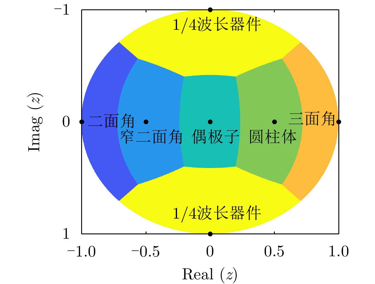
Figure 1. Unit disc representation of
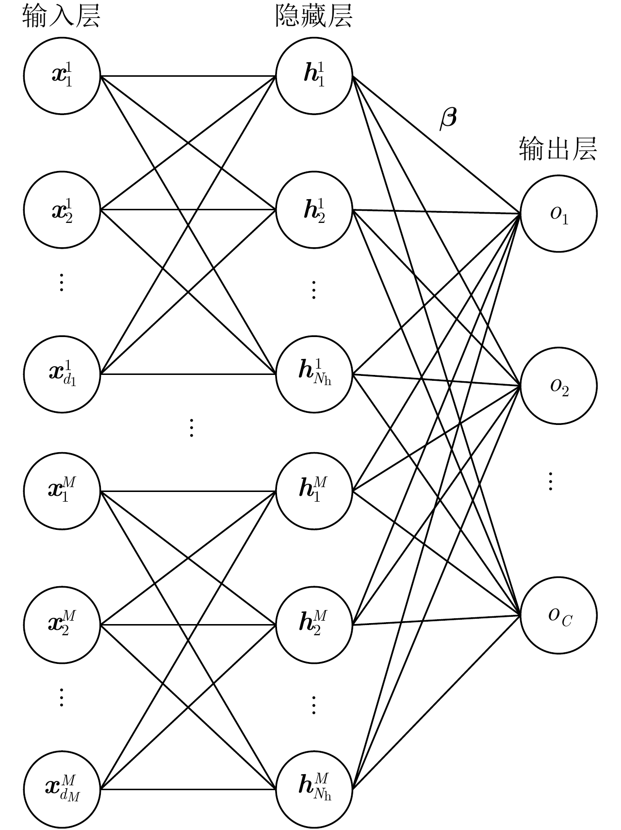
$z$ - Figure 2. Feature level fusing RKELM network based on prototype clustering preprocessing
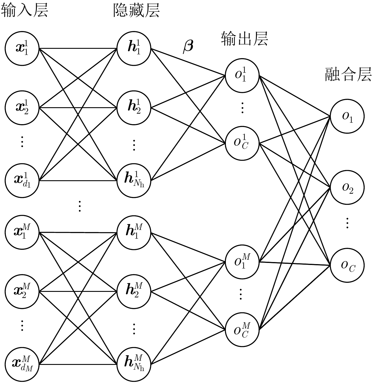
- Figure 3. Decision level fusing RKELM network based on prototype clustering preprocessing
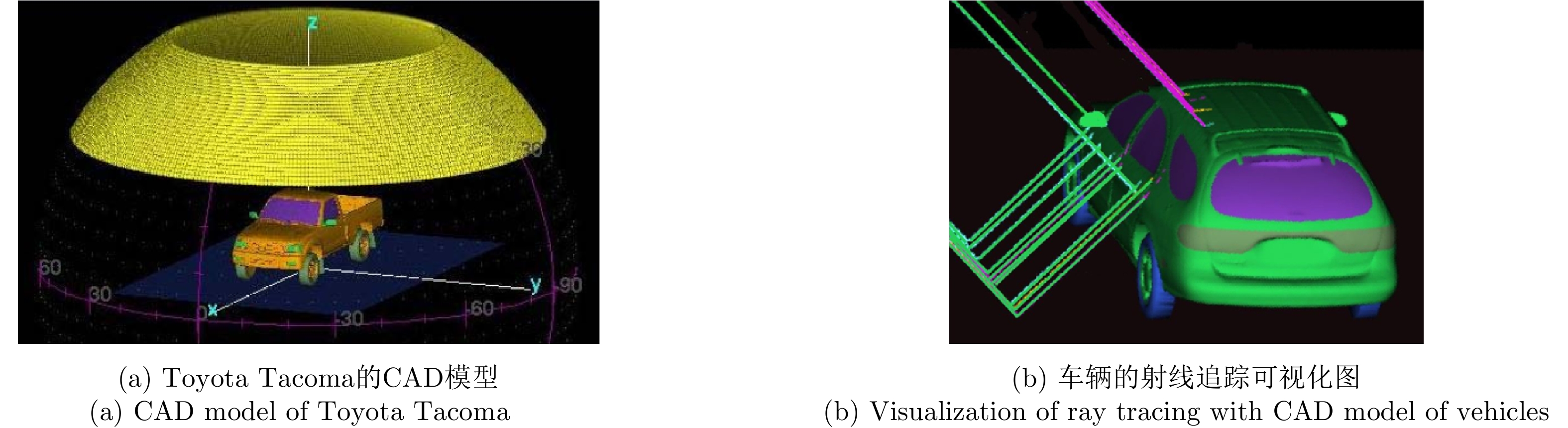
- Figure 4. Diagram of simulated echo from civilian vehicles
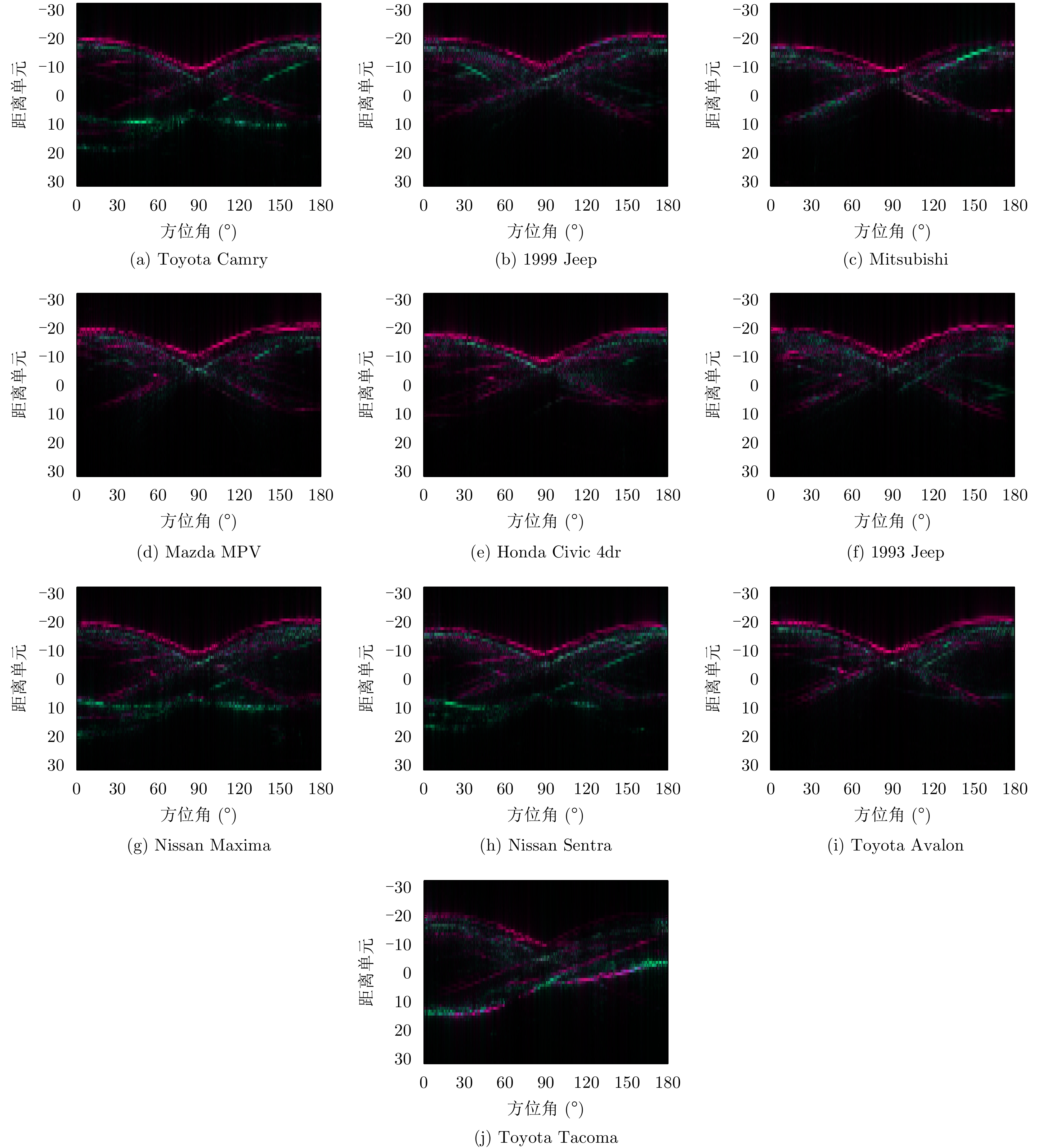
- Figure 5. RGB images of the Cameron projection features from 10 civilian vehicles
- Figure 6. Average recognition rates versus size of training data
- Figure 7. Average recognition rates versus SNR