Loading [MathJax]/jax/element/mml/optable/MathOperators.js
Lu Xinfei, Xia Jie, Yin Zhiping, et al.. High-resolution radar imaging using 2D deconvolution with sparse echo denoising[J]. Journal of Radars, 2018, 7(3): 285–293. DOI: 10.12000/JR17108
Citation: Lu Xinfei, Xia Jie, Yin Zhiping, et al.. High-resolution radar imaging using 2D deconvolution with sparse echo denoising[J]. Journal of Radars, 2018, 7(3): 285–293. DOI: 10.12000/JR17108

High-resolution Radar Imaging Using 2D Deconvolution with Sparse Echo Denoising

DOI: 10.12000/JR17108 CSTR: 32380.14.JR17108
Funds:  The National Natural Science Foundation of China (61401140).
More Information
  • Author Bio:

    Lu Xinfei (1990–) was born in Anhui, China. He received the B.E., M.E. and Ph.D. degrees both from University of Science and Technology of China (USTC), Hefei, China, in 2011, 2015 and 2017, respectively. His current research interests include MIMO imaging, ISAR imaging, compressed sensing, and signal reconstruction. E-mail: lxfei@mail.ustc.edu.cn

    Xia Jie (1993–) was born in Anhui, China. She is currently a master student in University of Science and Technology of China. She received her Bachelor degree in electronic engineering and information science from HeFei University of Technology. Her current research interests include forward-looking imaging, compressed sensing, and sparse signal reconstruction. E-mail: jiexia@mail.ustc.edu.cn

    Yin Zhiping (1980–) received his B.E. degree in electronic engineering and the Ph.D. degree in electromagnetic field and microwave technology from the University of Science and Technology of China (USTC), Hefei, China, in 2003 and 2008, respectively. From 2009 to 2010, he worked in the Microwave and Millimeter-wave Engineering Research Center, USTC, as a postdoctor. Now, he is an associate professor of the Academy of Photoelectric Technology, Hefei University of Technology, Hefei, China. His current research interests include microwave and terahertz device, phased-array antenna and microwave imaging radar. E-mail: zpyin@hfut.edu.cn

    Chen Weidong (1968–) received his B.E. degree from University of Electronic Science and Technology of China, in 1990, and the M.E. and Ph.D. degrees both from University of Science and Technology of China (USTC), Hefei, China, in 1994 and 2005, respectively. Since 1994, he was been with the Department of Electronic Engineering and Information Science, USTC, where he is now a professor. His research interests include microwave imaging, microwave and millimeter wave technology and system, and radar imaging. E-mail: wdchen@ustc.edu.cn

  • Corresponding author: Chen Weidong E-mail: wdchen@ustc.edu.cn
  • Received Date: 2017-11-20
  • Rev Recd Date: 2018-05-09
  • Available Online: 2018-06-22
  • Publish Date: 2018-06-01
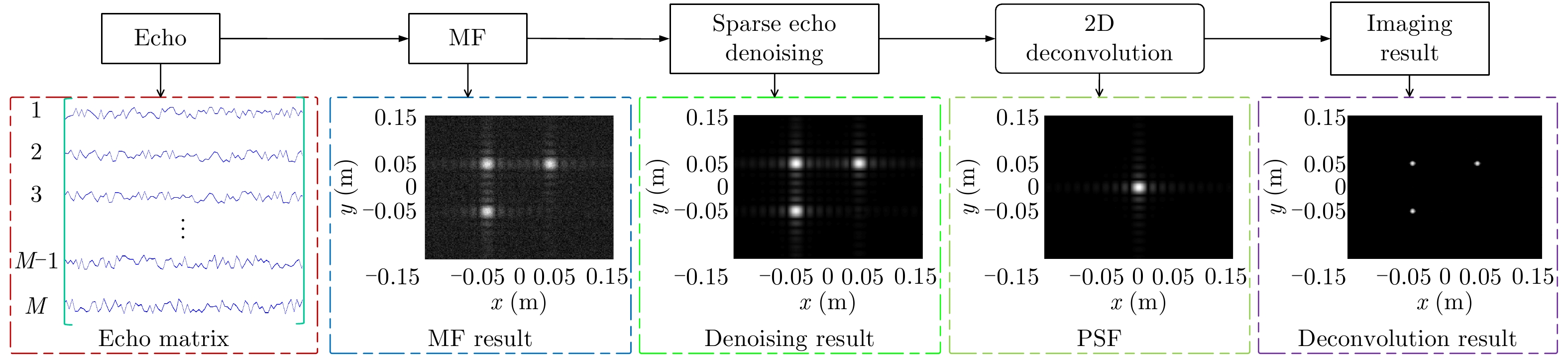
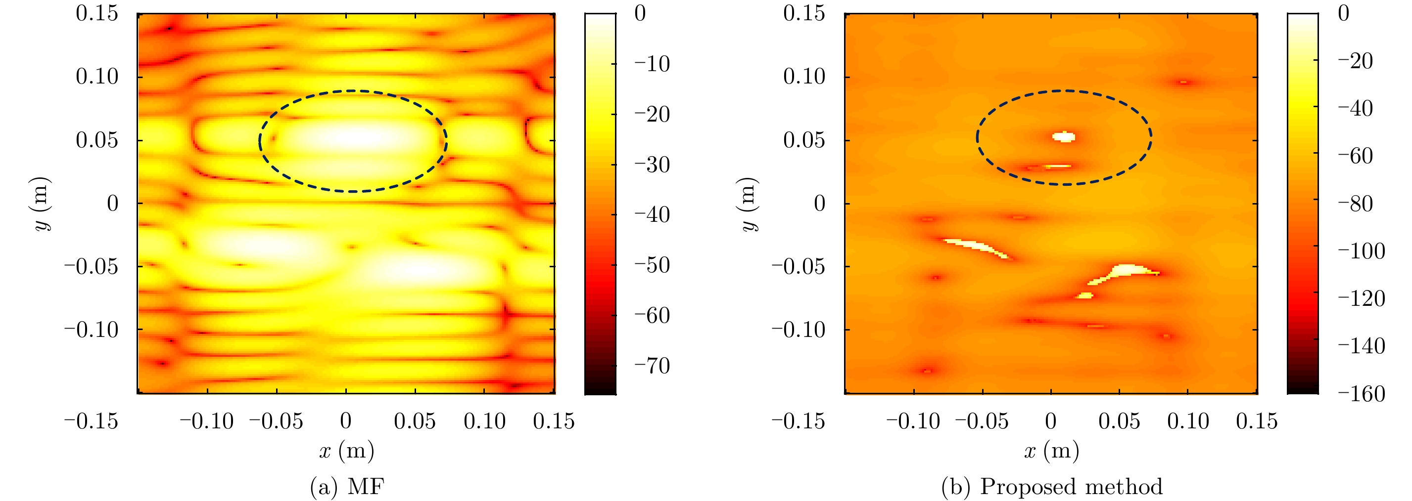
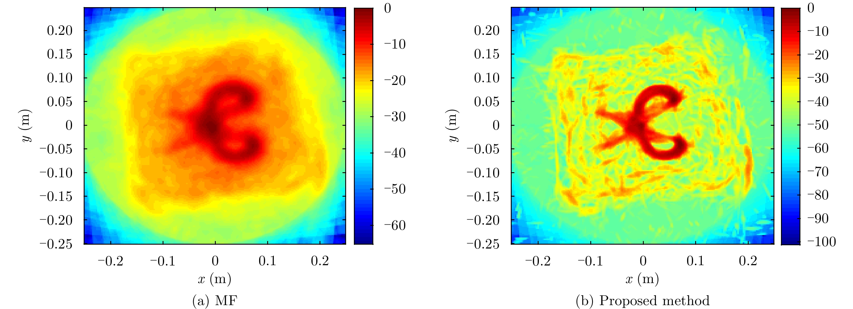
  • This study proposes a high-resolution radar imaging method combined with the sparse low-rank matrix recovery technique and the deconvolution algorithm based on the matched filtering result. We establish a two-Dimensional (2D) convolution model for the radar signal after the Matched Filter (MF) to maximize the Signal-to-Noise Ratio (SNR) and use the 2D deconvolution algorithm of the Wiener filter to obtain a high resolution. However, representative deconvolution algorithms are confronted with an ill-posed problem, which magnifies the noise while influencing the imaging resolution. Prior to this study, the echo matrix after the MF was proven to be sparse and low rank under the constraint of a sparsely distributed target. The target distribution is smoothed by the influence of the point spread function. Hence, inspired by these points, we further enhance the SNR of the echo matrix based on the sparse and low-rank characteristics to alleviate the ill-posed problem of deconvolution and the poor resolution of the Wiener filter. The performance of the proposed method is demonstrated by the real experimental data.


  • High resolution radar imaging has been widely used in target scattering diagnostics and recognition. As we all know, high resolution in range dimension is derived from the bandwidth of the transmitting signal and in the cross range dimension from synthetic aperture of multiple spatial positions. Under the fixed bandwidth and the synthetic aperture, traditional Matched Filter (MF) based methods for radar imaging suffer from low resolution and high sidelobes limited by the synthetic aperture[1].

    In order to improve the resolution and suppress the sidelobes, many high resolution methods have been applied to radar imaging. For example, the recently introduced theory of Compressed Sensing (CS) provides an idea to improve the resolution and reduce the amounts of measurement data under the constraint of sparsely distributed target prior, which has been widely explored for applications of radar imaging[24]. However, conventional CS methods are confronted with a range of problems in practical scenarios, such as complexity in calculation, high Signal-to-Noise Ratio (SNR) requirement, model mismatch caused by off grid problem[5], phase mismatch[6], frequency error[7] and position error[8]. To avoid the off grid problem of CS, modern spectral estimation methods like MUltiple SIgnal Classification (MUSIC), matrix pencil and Estimation of Signal Parameters via Rotational Invariance Techniques (ESPRIT) have been used in radar imaging for resolution improvement[9]. However, most those methods suffer from performance degradation when there is little prior knowledge of the exact numbers of the scatters or under low SNR condition. Recently, the atomic norm minimization algorithm[10] based on continuous compressed sensing is introduced to enhance the SNR of the received echo and using Vandermonde decomposition to eliminate the grid mismatch. Nevertheless, this method can only be tailored to a specific model and brings huge computational cost.

    Consideration the aforementioned fact while combining the sparsity low rank matrix recovery technology and deconvolution algorithm, we introduce a high resolution radar imaging method based on the MF result. Firstly we establish the convolution model of target’s backscatter coefficients and the Point Spread Function (PSF), and then we want to use the deconvolution method like Wiener filter to improve the radar imaging resolution. However, the performance improvements of those methods depend on high SNR, and their super resolution performance is visibly affected by the low pass character of the PSF[11]. Although the MF result has enhanced the SNR, we can further improve the echo SNR by the sparsity and low rank matrix recovery. Low rank matrix recovery has been applied in many signal processing applications to estimate a low rank matrix from its noisy observation[12, 13]. Combinng the sparsity of the echo matrix, we modify the low rank matrix recovery and introduce it to radar echo denoising, which can improve the performance of the two-Dimensional (2D) deconvolution. Finally, some experimental results are conducted to verify the effectiveness of the proposed method.

    Notation: (·)T, (·)H and (·)* denote the transpose, the conjugate transpose and the conjugate operation, respectively. ,﹡, and ☉ indicate the inner product, the convolution and the Hadamard product. F, 1, are the Frobenius norm, sum of the absolute values and the nuclear norm.

    Considering a typical arrangement for radar imaging in which an object with scattering reflectivity σxy rotated by a scan angle θm (as shown in Fig. 1), we defined the positions of the transmitting and receiving antenna shown in a Cartesian coordinate as (W/2, –R, H) and (–W/2, –R,H), where W, R, H represent the antenna spacing, distance from antenna to XZ plane and XY plane, respectively.

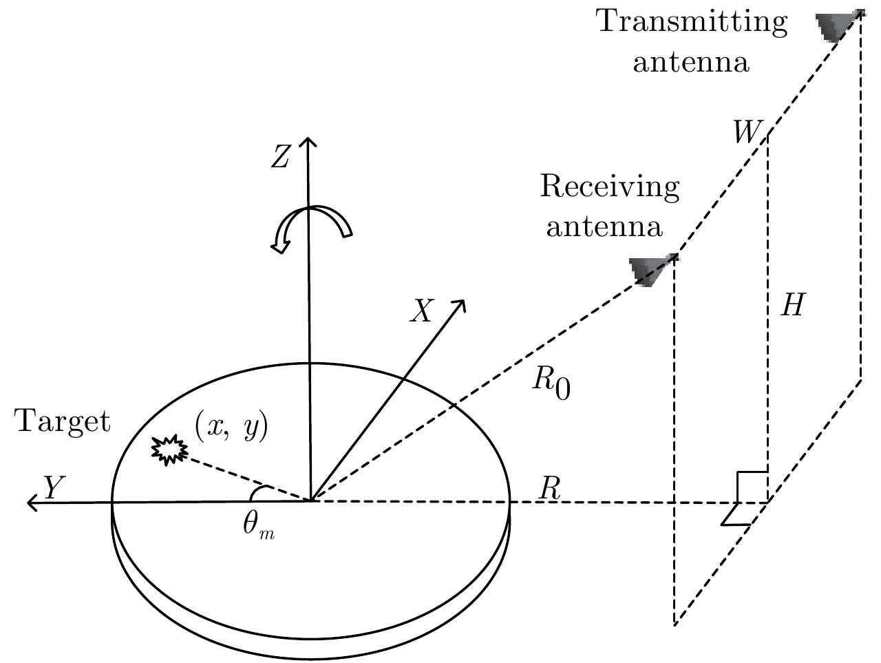
    Figure  1.  Radar imaging geometry

    Transmitting a stepped-frequency signal with frequency fn and under Born approximation, the received scattered echo with Gauss noise Wmn is given by:

    Ymn= (1)

    In this equation: {f_{\!n}} = {f_0} + n\Delta f,n = 0,1 ·\!·· ,N - 1, {f_0} and \Delta f represent the start frequency and frequency step, {\theta _m} = m\Delta \theta ,m = 0,1, ·\!·\!· ,M, \Delta \theta represents the rotating angle step, respectively. The range R\left( {x,y;{\theta _m}} \right) from the transmitting antenna to echo scattering center and to the receiving antenna can be calculated as Eq. (2):

    \begin{align} R\left( {x,y;{\theta _m}} \right) = & \sqrt {{{\left( {x\cos {\theta _m} - y\sin {\theta _m} + \frac{W}{2}} \right)}^2} + {{\left( {x\sin {\theta _m} + y\cos {\theta _m} + R} \right)}^2} + {H^2}} \\ & + \sqrt {{{\left( {x\cos {\theta _m} - y\sin {\theta _m} - \frac{W}{2}} \right)}^2} + {{\left( {x\sin {\theta _m} + y\cos {\theta _m} + R} \right)}^2} + {H^2}} \end{align} (2)

    In far-field and small rotation angle case, R\left( {x,y;{\theta _m}} \right) can be approximated by first order Taylor-series expansion as:

    R\left( {x,y;{\theta _m}} \right) \approx 2 \Big( {{R_0} + \left( {x + m\Delta \theta y} \right)R/{R_0}} \Big) (3)

    where {R_0} = \sqrt {{R^2} + {{\left( {W/2} \right)}^2} + {H^2}} .

    Then the received echo can be written as follow under some approximated conditions:

    {{\tilde Y}_{mn}} =\!\! \iint\limits_S {{{\tilde \sigma }_{xy}}{{\rm{e}}^{ - {\rm{j4}} {\text{π}} \scriptsize\displaystyle\frac{{R\Delta \theta }}{{\lambda {R_0}}}mx}}{{\rm{e}}^{ - {\rm{j}}4{\text{π}} \scriptsize\displaystyle\frac{{R\Delta f}}{{{R_0}c}}ny}}{\rm{d}}x{\rm{d}}y} + {W_{mn}} (4)

    where {\tilde \sigma _{xy}} \!\!=\!\! {\sigma _{xy}}{{\rm{e}}^{ - {\rm{j}}4{\text{π}} Ry/\!\lambda {R_0}}}, \;\;{{{\tilde Y} }_{mn}} \!\!=\!\!\! {Y_{mn}}{{\rm{e}}^{{\rm{j}}4{\text{π}} {f_{\!n}}{R_0}/\!c}}, \lambda \!\!\approx\!\! c/\!{f_0}.

    After discrete imaging region with P×Q grids, the received echo in Eq. (4) can be described as the following 2D linear signal model:

    {\tilde{{\text{Y}}}} = {{\text{A}}_x}\tilde{{\text{Σ}} }{\text{A}}_y^{\rm T} + {\text{W}} (5)

    where {\tilde{\text{Y}}} \!\!=\!\! {\left[ \ \ {{{\tilde {Y}}_{mn}}} \right]_{M \times N}} is the echo matrix, \tilde{{\text{Σ}} } \!=\! {\left[ {{{\tilde \sigma }_{pq}}} \right]_{P \times Q}} is the observation matrix: {{{\text{A}}}_x} = {\left[ {{{\rm{e}}^{ - {\rm{j}}4{\text{π}} m{x_p}R\Delta \theta /\lambda {R_0}}}} \right]_{M \times P}}, {{{\text{A}}}_y} = {\left[ {{{\rm{e}}^{ - {\rm{j}}4{\text{π}} n{y_q}R\Delta f/{R_0}c}}} \right]_{N \times Q}}.

    Considering the targets present sparse point scattering characteristic under high frequency scattering in most practical application scenarios, we present our method to improve the resolution of radar imaging under sparse target constraint using 2D deconvolution algorithm with low rank sparsity echo matrix denoising.

    As we all know, the MF algorithm which is based on the maximum signal to noise ratio is the most stable and commonly used radar imaging method. However, due to limitation of the synthetic aperture and bandwidth, the standard MF method suffers from relatively low resolution and high sidelobes, especially under the requirements of high resolution. The received echo after MF from Eq. (5) can be obtained by:

    {{{\text{Y}}}_{\! {\rm MF}}} = {{\text{A}}}_x^{{\rm H}}\ \ {\tilde{ \text{Y}} }{\text{A}}_y^* (6)

    From the result of Eq. (6), the echo of the surface target after MF can be described as the sum of all the wave scattered at the points on the surface grid, i.e.,

    {{{\text{Y}}}_{\rm {\!MF}}}\left( {x,y} \right) = \sum\limits_{x'}^{} {\sum\limits_{y'}^{} {\tilde \sigma \left( {x',y'} \right){P_{sf}}\left( {x - x',y - y'} \right)} } (7)

    where we define the PSF as:

    {P_{sf}}\left( {x \!-\!\! x',y \!-\!\! y'} \right) \!=\!\! \left\langle {{{\text{a}}_x}\left( x \right),{{\text{a}}_x}\left( {x'} \right)} \right\rangle\! \left\langle {{{\text{a}}_y}\left( y \right),{{\text{a}}_y}\left( {y'} \right)} \right\rangle \hspace{20pt} (8)

    here, {{\text{a}}_x}\left( x \right) and {{\text{a}}_y}\left( y \right) represent the column of matrix Ax and Ay at the grid (x, y).

    We can find that Eq. (6) can be seen as the 2D convolution of the PSF and target backscatter coefficients:

    {{{\text{Y}}}_{\!\rm MF}}\left( {x,y} \right) = \tilde \sigma \left( {x,y} \right)*{P_{sf}}\left( {x,y} \right) + {W_{\rm MF}}\left( {x,y} \right) (9)

    Inspired by this, we can recovery the backscatter coefficients using deconvolution algorithm to improve the imaging quality. Firstly, we should analyze the characteristic of the PSF and its influence on the deconvolution result.

    The PSF can be evaluated as:

    \begin{align} {P_{sf}}\left( {x,y} \right) \approx & {{\rm{e}}^{ - {\rm{j}}2{\text{π}} \left[ {\scriptsize\displaystyle\frac{{\left( {M - 1} \right)R\Delta \theta }}{{\lambda {R_0}}}x + \scriptsize\displaystyle\frac{{\left( {N - 1} \right)R\Delta f}}{{{R_0}c}}y} \right]}} \\ &\cdot \operatorname{sinc} \left( {\frac{{2MR\Delta \theta }}{{\lambda {R_0}}}x} \right)\operatorname{sinc} \left( {\frac{{2NR\Delta f}}{{{R_0}c}}y} \right) \end{align}

    (10)

    We can calculate the 2D mainlobe width which represents the radar imaging resolution as follows:

    {\rho _x} = \frac{{\lambda {R_0}}}{{2MR\Delta \theta }},\;\;\;{\rho _y} = \frac{{{R_0}c}}{{2NR\Delta f}} (11)

    Eq. (9) indicates that the MF result can be seen as the convolution result of backscatter coefficients and {P_{sf}}\left( {x,y} \right). The PSF is characterized by synthetic aperture and bandwidth, which has strong low pass characteristic with low resolution and high sidelobes as shown in Eq. (10) and Eq. (11). For an isolated target scatter, imaging result after the MF output will be proportional to the PSF, therefore the resolution of MF result is limited and accompanied by low resolution and high sidelobes. Inspired by above, we can restore the high resolution backscatter coefficients information by deconvolution to remove the effect of low pass characteristic of PSF.

    As we have get 2D convolution form as Eq. (9), here we consider to use the direct deconvolution algorithm to recovery target backscatter coefficients. Firstly, we transform Eq. (9) into the spatial frequency domain using 2D Fourier transform as:

    {{{\text{Y}}}_{\!\omega} } = {{\text{Σ}}_{\!\omega} } \odot {{{\text{H}}}_{\!\omega}}\;{\omega} + {{{\text{W}}}_{\!\omega} } (12)

    where, {{{\text{Y}}}_{\!\omega} } \!=\!\! \mathcal{F}\left\{ {{{{\text{Y}}}_{\!\!{\rm {MF}}}}} \right\},{{\text{Σ}}_\omega } \!=\!\! \mathcal{F}\left\{ {\tilde{{\text{Σ}} }} \right\},{{{\text{H}}}_\omega } \!=\!\! \mathcal{F}\left\{ {{{{\text{P}}}_{\!\!sf}}} \right\}, {{{\text{W}}}_{\!\!\omega} } \!=\! \mathcal{F}\left\{ {{{{\text{W}}}_{\!\!{\rm {MF}}}}} \right\}.

    Theoretically, the target scattering information could be restored by deconvolution as:

    {{\text{Σ}}_\omega } = {{{\text{Y}}}_{\!\!\omega} }/{{{\text{H}}}_\omega } (13)

    However, 1/{{{\text{H}}}_\omega } will be very large in practice at the outside of the mainlobe of PSF since the low pass characteristic of the PSF, which results in tremendous amplification of noise and obtains valueless results. So the deconvolution processing becomes an ill-posed inverse problem.

    In order to alleviate the ill-posed problem, we use Winner filtering algorithm and sparse low rank matrix recovery to improve the quality of imaging result.

    The result after Winner filter algorithm can be written as[14]:

    {\tilde{{\text{Σ}} }_\omega } = {{{\text{Y}}}_{\!\!\omega} } \odot \frac{{{{{\text{H}}}_\omega }\!\!^*}}{{{{\left\| {{{{\text{H}}}_\omega }} \right\|}^2} + {\Psi _{\rm WW}}\left( \omega \right)/{\Psi _{\Sigma \Sigma }}\left( \omega \right)}} (14)

    where {\Psi _{\rm WW}}\left( \omega \right) and {\Psi _{\Sigma \Sigma }}\left( \omega \right) is the power spectral density of {{\text{W}}} and {\text{Σ}}. Eq. (14) will approach Eq. (13) when the SNR is relatively high. What’s more, Eq. (14) will attenuate the high frequencies noise to alleviate the ill-posed problem under low SNR. In experimental data processing, the {\Psi _{\rm WW}}\left( \omega \right)/{\Psi _{\Sigma \Sigma }}\left( \omega \right) is generally set according to the experience value. We can get the scattering reflectivity \tilde{{\text{Σ}} } by 2D Inverse Fourier transform according to Eq. (14).

    We can prove that the echo matrix after MF is sparse and low rank in Appendix A and by using this characteristic, the echo SNR can be improved. Consider the problem of estimating a sparse low rank matrix X from its noisy observation Y:

    {{\text{Y}}} = {{\text{X}}} + {{\text{W}}} (15)

    Define the sparse low rank matrix recovery problem as:

    \begin{align} &\mathop {\min }\limits_{{\text{X}},{\text{D}}} \;\gamma {\left\| {\text{X}} \right\|_*} + \left( {1 - \gamma } \right){\left\| {\text{D}} \right\|_1}{\rm{subject}}\;{\rm{to}}\\ &{\text{Y}} = {\text{X}} + {\text{W}},{\text{D}} = {\text{X}} \end{align} (16)

    where \gamma is the regularization parameter used to balance the relative contribution between nuclear norm and the 1-norm, which can control the denoising performance. In general, the denoising threshold of \gamma can be set as the 5%~10% of the maximum singular value of Y.

    By applying Augmented Lagrangian Method (ALM), we can get the optimization problem:

    \begin{align} F\left( {{{\text{X}}},{{\text{D}}},{{{\text{Y}}}_{\!1}},{{{\text{Y}}}_{\!2}},\mu } \right) \!=\! & \gamma {\left\| {{\text{X}}} \right\|_*} + \left\langle {{{{\text{Y}}}_{\!1}},{{\text{Y}}} - {{\text{X}}}} \right\rangle \\ &+\! \frac{\mu }{2}\left\| {{{\text{Y}}} \!-\! {{\text{X}}}} \right\|_F^2 \!+\! \left( {1 \!-\!\! \gamma } \right){\left\| {{\text{D}}} \right\|_1} \\ &+\! \left\langle {{{{\text{Y}}}_2},{{\text{D}}} - {{\text{X}}}} \right\rangle \!\!+\!\! \frac{\mu }{2}\left\| {{{\text{D}}} \!\!-\!\! {{\text{X}}}} \right\|_F^2 \end{align}

    (17)

    And the update rules for solving this problem are as follows:

    {{{\text{X}}}^{\left( {k + 1} \right)}} = \mathcal{S}\left( {\frac{{{{\text{Y}}} \!\!+\!\! {{{\text{D}}}^{\left( k \right)}}}}{2} \!+\! \frac{{{{\text{Y}}}_1^{\left( k \right)} \!+\! {{\text{Y}}}_2^{\left( k \right)}}}{{2{\mu ^{\left( k \right)}}}},\frac{\gamma }{{2{\mu ^{\left( k \right)}}}}} \right) (18)
    {{{\text{D}}}^{\left( {k + 1} \right)}} = {\rm{soft}}\left( {\frac{1}{{{\mu ^{\left( k \right)}}}}{{\text{Y}}}_2^{\left( k \right)} - {{{\text{X}}}^{\left( {k + 1} \right)}},\frac{{1 - \gamma }}{{{\mu ^{\left( k \right)}}}}} \right)\quad (19)
    \!\!\!\!\!\!\!\!\!\!\left. \begin{align} {{\text{Y}}}_1^{\left( {k + 1} \right)} =& {{\text{Y}}}_1^{\left( k \right)} + {\mu ^{\left( k \right)}}\left( {{{\text{Y}}} - {{{\text{X}}}^{\left( {k + 1} \right)}}} \right) \\ {{\text{Y}}}_2^{\left( {k + 1} \right)} =& {{\text{Y}}}_2^{\left( k \right)} + {\mu ^{\left( k \right)}}\left( {{{{\text{D}}}^{\left( {k + 1} \right)}} - {{{\text{X}}}^{\left( {k + 1} \right)}}} \right) \quad\; \\ {\mu ^{\left( {k + 1} \right)}} =& \beta {\mu ^{\left( k \right)}},\,\,\, \beta > 1 \end{align}\!\!\!\!\!\!\right\} (20)

    where, \mathcal{S}\left( { \cdot , \cdot } \right) is the singular value thresholding function defined as:

    \mathcal{S}\left( {{{\text{X}}},\gamma } \right){\rm{ = }}{{\text{U}}}{\rm{soft}}\left( {{\text{Σ}},\gamma } \right){{{\text{V}}}^{\rm T}} (21)

    where, {{\text{X}}} = {{\text{U}}}{\text{Σ}}{{{\text{V}}}^{\rm T}\,} is the Singular Value Decomposition (SVD) of {{\text{X}}}, {\rm{soft}}\left( \cdot \right) is the soft thresholding function defined as:

    {\rm{soft}}\left( {x,\gamma } \right) = {\rm{sign}}\left( x \right) \cdot \max \left\{ {\left| x \right| - \gamma ,0} \right\} (22)

    See Appendix B for the detailed derivation of Eq. (18) and Eq. (19).

    The flowchart of the proposed method is shown in Fig. 2 by combining the sparse low rank matrix recovery with the 2D deconvolution.

    Figure  2.  The flowchart of the proposed method

    The parameters in the simulation are given in Tab. 1. In this experiment, we set four-point targets, the imaging results are shown in Fig. 3.

    Table  1.  Simulation parameters
    ParameterValueParameterValue
    {{M}}256R1 m
    {{N}}500H0.7 m
    \Delta f10 MHzW0.04 m
    \Delta \theta 0.009°SNR–15 dB
     | Show Table
    DownLoad: CSV
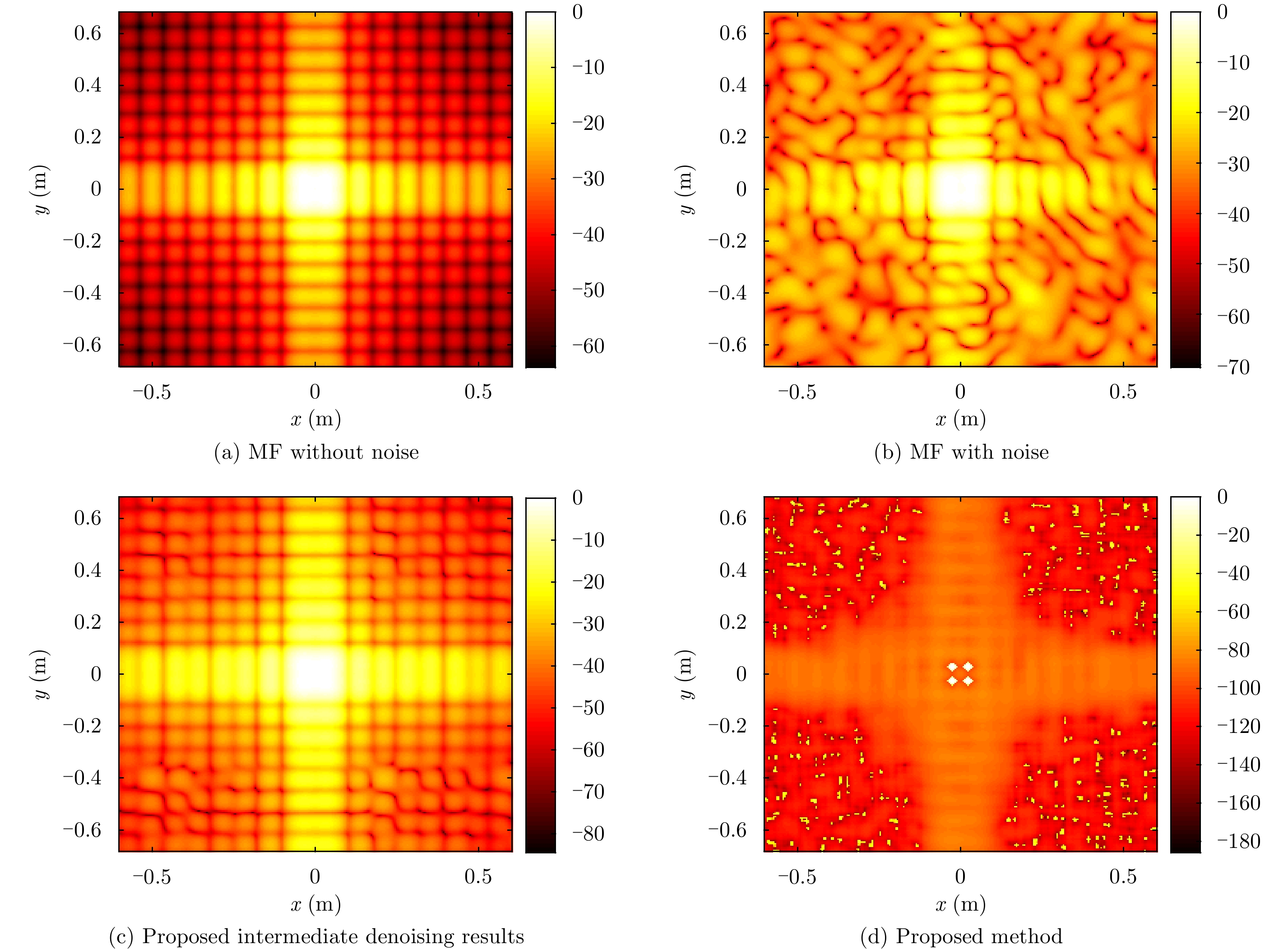
    Figure  3.  Imaging results

    As shown in Fig. 3(a), due to the limitation of synthetic aperture and bandwidth, the MF method suffers from relatively low resolution and high sidelobes which make it difficult to distinguish between four-point targets even there is no noise. Fig. 3(b)Fig. 3(d) show the imaging results reconstructed by MF and proposed method including the intermediate denoising results when SNR = –15 dB. It can be clearly seen that the effect of denoising compared Fig. 3(c) with Fig. 3(a) and Fig. 3(b), the echo SNR is further improved by the sparsity and low rank matrix recovery during the proposed intermediate denoising procedure. The final imaging result is shown in Fig. 3(d), from which we can see that the proposed method has a better reconstruction precision with higher resolution imaging of four distinguishable point targets.

    The experimental scene is shown in Fig. 4(a), which is the same with the model in Fig. 1. The radar system consists of a pair of horn antennas, a turntable whose rotation angle can be precisely controlled by the computer, and an Agilent VNA N5224A which is used for transmitting and receiving the stepped-frequency signal with bandwidth of 10 GHz from 28 GHz to 38 GHz and number of frequencies N equals to 256 (Frequency interval \Delta f is 40 MHz). Two kind of targets including three 5-mm-diameter mental spheres and a pair of scissors placed on a rotatory platform are used here as shown in Fig. 4(b).

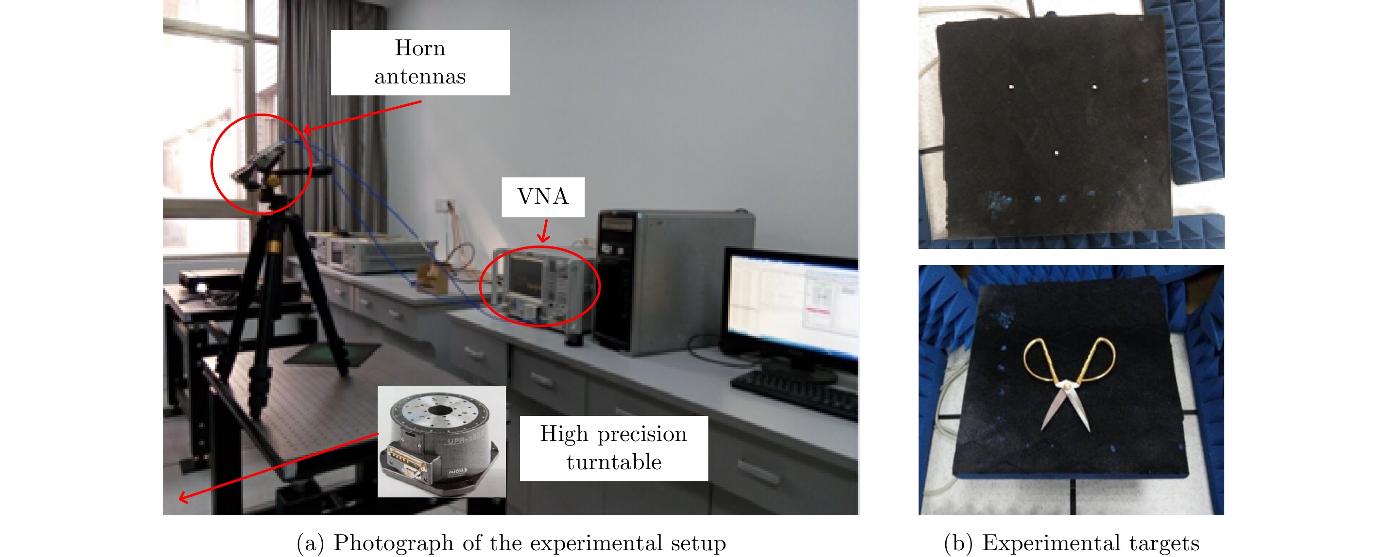
    Figure  4.  Experimental scene VNA

    As we know, image entropy can be considered as a metric for measuring the smoothness of the probability density function of image intensities[15]. The imaging entropy is defined as:

    E\left( I \right) = - \sum\limits_{p = 1}^P {\sum\limits_{q = 1}^Q {\left| {\frac{{{I^2}\left( {p,q} \right)}}{{s\left( I \right)}}} \right| \ln \left| {\frac{{{I^2}\left( {p,q} \right)}}{{s\left( I \right)}}} \right|} } (23)

    where s\left( I \right) = \displaystyle\sum\nolimits_{p = 1}^P {\sum\nolimits_{q = 1}^Q {{{\left| {I\left( {p,q} \right)} \right|}^2}} } .

    In this experiment, we set R \!=\! 1\;{\rm m},\ H \!=\! 0.7\;{\rm m},W = 0.04\;{\rm m} and the total rotating angle is {5^ \circ } with an angle interval \Delta \theta = {0.01^ \circ } (M = 500).

    Fig. 5 shows the results of the MF and our proposed method for the mental spheres. The one-dimensional x and y domain cross-section of the target with red-dashed circle shown in Fig. 5 are presented in Fig. 6, in which the red-dashed line and blue line represent the result of MF and proposed method. Clearly, the reconstruction result of proposed method has a narrower main-lobe and lower side-lobe than MF and the sharpening ratio almost reach 5.8 and 3.0 in x and y domain, respectively.

    Figure  5.  Imaging results of mental spheres
    Figure  6.  One-dimensional cut through the target with red dashed circle in Fig. 5

    The parameters for this experiment are set as follows, R = 0.876\;{\rm m}, W = 0.04\;{\rm m}. The total rotating angle is {360^ \circ } with M equals to {720^ \circ }. Taking into account the scintillation characteristics of the target under large rotating angle, we divide the rotating angle into 72 segments and each of the part is with rotating angle from {0^ \circ } to {5^ \circ }. The proposed method is used to process the data for each segment and the image fusion method is used to merge the results of all segments.

    Fig. 7 shows the imaging results of the scissors reconstructed by MF and proposed method. It can be seen from the results that the proposed method has a high reconstruction precision with a shaper shape of scissors.

    Figure  7.  Imaging results of scissors

    The entropies of the imaging results by MF and our proposed method are given in Tab. 2 to quantitatively assess the performance. The proposed method has a low entropy which means the proposed method can improve the resolution and verifies its superiority.

    Table  2.  Entropies of imaging results
    TargetMFOur proposed method
    Mental spheres8.72824.8429
    Scissors8.94337.0454
     | Show Table
    DownLoad: CSV

    We introduce a robust deconvolution method with enhancing SNR technology to realize high resolution radar imaging. Compared to other high resolution methods, our proposed method is simple and robust. Although the signal model and experiments are performed for turntable radar situation with SF waveform, the method can be directly generalized to other practical radar systems based on other types of signals.

    Appendix A Proof of the sparsity and low rank characteristic

    To prove the echo matrix after MF is sparse and low rank, the following lemma is needed.

    Lemma 1[16]: For matrix A and B, the ranks of the product of A and B satisfy the inequality below:

    {\rm{rank}}\left( {{{\text{AB}}}} \right) \le \min \left\{ {{\rm{rank}}\left( {{\text{A}}} \right),{\rm{rank}}\left( {{\text{B}}} \right)} \right\} (A-1)

    From Eq. (5) and Eq. (6), we can see that the echo matrix after MF can be written as:

    {{{\text{Y}}}_{\!\!{\rm {MF}}}} \ = {{\text{A}}}_x^{\rm H}{{{\text{A}}}_x}\tilde{{\text{Σ}} }{{\text{A}}}_y^{\rm T}{{\text{A}}}_y^* (A-2)

    We have supposed that the target has sparse distribution, so the target backscatter coefficients matrix \tilde{{\text{Σ}} } is sparse and low rank. Thus, matrix {{{\text{Y}}}_{{\!\rm{MF}}}} is also low rank according to lemma 1. The sparsity of matrix {{{\text{Y}}}_{{\rm{\!\!MF}}}} can be proved by Eq. (9) obviously.

    Appendix B Derivation of Eq. (18) and Eq. (19)

    For Eq. (18), the optimization problem can be described as Eq. (B-1), and it has a closed-form solution just as Eq. (18) according to Ref. [13].

    \begin{align} {{{\text{X}}}^{\left( {k + 1} \right)}}\!\!\!\!\!\!\!\!\!\!\! & \\ & =\!\! \arg \mathop {\min }\limits_{{\text{X}}} F\left( {{{\text{X}}},{{{\text{D}}}^{\left( k \right)}},{{\text{Y}}}_1^{\left( k \right)},{{\text{Y}}}_2^{\left( k \right)},{\mu ^{\left( k \right)}}} \right) \\ & =\!\! \arg \mathop {\min }\limits_{{\text{X}}} \frac{1}{2}\left\| {{\text{X}}} \!- \! \frac{1}{2}\left( {{{\text{Y}}} \!+\! {{{\text{D}}}^{\left( k \right)}} \!+\! \frac{{\text{Y}}_1^{\left( k \right)}\!+\!\! {{\text{Y}}}_2^{\left( k \right)}}{{{\mu ^{\left( k \right)}}}}} \right) \right\|_F^2 \\ &\quad + \frac{\gamma }{{2{\mu ^{\left( k \right)}}}}{\left\| {{\text{X}}} \right\|_*} \end{align} (B-1)

    For Eq. (19), it is the same with Eq. (18), which can written as

    \begin{align} {{{\text{D}}}^{\left( {k + 1} \right)}} = & \arg \mathop {\min }\limits_{{\text{D}}} F\left( {{{{\text{X}}}^{\left( {k + 1} \right)}},{{\text{D}}},{{\text{Y}}}_1^{\left( k \right)},{{\text{Y}}}_2^{\left( k \right)},{\mu ^{\left( k \right)}}} \right) \\ = & \arg \mathop {\min }\limits_{{\text{D}}} \frac{1}{2}\left\| {{{\text{D}}} - \left( {\frac{{{{\text{Y}}}_2^{\left( k \right)}}}{{{\mu ^{\left( k \right)}}}} - {{{\text{X}}}^{\left( {k + 1} \right)}}} \right)} \right\|_F^2 \\ &+ \frac{{1 - \gamma }}{{{\mu ^{\left( k \right)}}}}{\left\| {{\text{D}}} \right\|_1} \end{align} (B-2)

    It also has a closed-form solution as Eq. (19) according to Ref. [17].

  • [1]
    Hu K B, Zhang X L, Shi J, et al. A novel synthetic bandwidth method based on BP imaging for stepped-frequency SAR[J]. Remote Sensing Letters, 2016, 7(8): 741–750.
    [2]
    Yiğit E. Compressed sensing for millimeter-wave ground based SAR/ISAR imaging[J]. Journal of Infrared, Millimeter, and Terahertz Waves, 2014, 35(11): 932–948.
    [3]
    Zhang S S, Zhang W, Zong Z L, et al. High-resolution bistatic ISAR imaging based on two-dimensional compressed sensing[J]. IEEE Transactions on Antennas and Propagation, 2015, 63(5): 2098–2111. DOI: 10.1109/TAP.2015.2408337.
    [4]
    Kreucher C and Brennan M. A compressive sensing approach to multistatic radar change imaging[J]. IEEE Transactions on Geoscience and Remote Sensing, 2014, 52(2): 1107–1112. DOI: 10.1109/TGRS.2013.2247408.
    [5]
    Wang T Y, Lu X F, Yu X F, et al. A fast and accurate sparse continuous signal reconstruction by homotopy DCD with non-convex regularization[J]. Sensors, 2014, 14(4): 5929–5951. DOI: 10.3390/s140405929.
    [6]
    Ding L and Chen W D. MIMO radar sparse imaging with phase mismatch[J]. IEEE Geoscience and Remote Sensing Letters, 2015, 12(4): 816–820. DOI: 10.1109/LGRS.2014.2363110.
    [7]
    Ding L, Chen W D, Zhang W Y, et al. MIMO radar imaging with imperfect carrier synchronization: A point spread function analysis[J]. IEEE Transactions on Aerospace and Electronic Systems, 2015, 51(3): 2236–2247. DOI: 10.1109/TAES.2015.140428.
    [8]
    Liu C C and Chen W D. Sparse self-calibration imaging via iterative MAP in FM-based distributed passive radar[J]. IEEE Geoscience and Remote Sensing Letters, 2013, 10(3): 538–542. DOI: 10.1109/LGRS.2012.2212272.
    [9]
    Wang X, Zhang M, and Zhao J. Efficient cross-range scaling method via two-dimensional unitary ESPRIT scattering center extraction algorithm[J]. IEEE Geoscience and Remote Sensing Letters, 2015, 12(5): 928–932. DOI: 10.1109/LGRS.2014.2367521.
    [10]
    Yang L, Zhou J X, Xiao H T, et al.. Two-dimensional radar imaging based on continuous compressed sensing[C]. Proceedings of the 5th Asia-Pacific Conference on Synthetic Aperture Radar (APSAR), Singapore, 2015: 710–713. DOI: 10.1109/APSAR.2015.730630.
    [11]
    Guan J C, Yang J Y, Huang Y L, et al. Maximum a posteriori-based angular superresolution for scanning radar imaging[J]. IEEE Transactions on Aerospace and Electronic Systems, 2014, 50(3): 2389–2398. DOI: 10.1109/TAES.2014.120555.
    [12]
    Parekh A and Selesnick I W. Enhanced low-rank matrix approximation[J]. IEEE Signal Processing Letters, 2016, 23(4): 493–497. DOI: 10.1109/LSP.2016.2535227.
    [13]
    Lin Z C, Chen M M, and Ma Y. The augmented lagrange multiplier method for exact recovery of corrupted low-rank matrices[R]. arXiv preprint arXiv:1009.5055, 2010. DOI: 10.1016/j.jsb.2012.10.010.
    [14]
    Pedone M, Bayro-Corrochano E, Flusser J, et al. Quaternion wiener deconvolution for noise robust color image registration[J]. IEEE Signal Processing Letters, 2015, 22(9): 1278–1282. DOI: 10.1109/LSP.2015.2398033.
    [15]
    Zhu J, Zhu S Q, and Liao G S. High-resolution radar imaging of space debris based on sparse representation[J]. IEEE Geoscience and Remote Sensing Letters, 2015, 12(10): 2090–2094. DOI: 10.1109/LGRS.2015.2449861.
    [16]
    Horn R A and Johnson C R. Matrix Analysis[M]. Cambridge: Cambridge University Press, 1990.
    [17]
    Donoho D L. De-noising by soft-thresholding[J]. IEEE Transactions on Information Theory, 1995, 41(3): 613–627. DOI: 10.1109/18.382009.
  • 加载中

Catalog

    通讯作者: 陈斌, bchen63@163.com
    • 1. 

      沈阳化工大学材料科学与工程学院 沈阳 110142

    1. 本站搜索
    2. 百度学术搜索
    3. 万方数据库搜索
    4. CNKI搜索

    Figures(7)  / Tables(2)

    Article views(3604) PDF downloads(347) Cited by()
    Proportional views
    Related

    /

    DownLoad:  Full-Size Img  PowerPoint
    • Table  1.  Simulation parameters
      ParameterValueParameterValue
      {{M}}256R1 m
      {{N}}500H0.7 m
      \Delta f10 MHzW0.04 m
      \Delta \theta 0.009°SNR–15 dB
       | Show Table
      DownLoad: CSV
    • Table  2.  Entropies of imaging results
      TargetMFOur proposed method
      Mental spheres8.72824.8429
      Scissors8.94337.0454
       | Show Table
      DownLoad: CSV