
 Submit Manuscript
 Peer Review
 Editor Work
- Home
- Articles & Issues
-
Data
- Dataset of Radar Detecting Sea
- SAR Dataset
- SARGroundObjectsTypes
- SARMV3D
- AIRSAT Constellation SAR Land Cover Classification Dataset
- 3DRIED
- UWB-HA4D
- LLS-LFMCWR
- FAIR-CSAR
- MSAR
- SDD-SAR
- FUSAR
- SpaceborneSAR3Dimaging
- Sea-land Segmentation
- SAR Multi-domain Ship Detection Dataset
- SAR-Airport
- Hilly and mountainous farmland time-series SAR and ground quadrat dataset
- SAR images for interference detection and suppression
- HP-SAR Evaluation & Analytical Dataset
- GDHuiYan-ATRNet
- Multi-System Maritime Low Observable Target Dataset
- DatasetinthePaper
- DatasetintheCompetition
- Report
- Course
- About
- Publish
- Editorial Board
- Chinese

| Citation: | 
|
Imaging Method for Co-prime-sampling Space-borne SAR Based on 2D Sparse-signal Reconstruction
DOI: 10.12000/JR19086 CSTR: 32380.14.JR19086
More Information-
Abstract
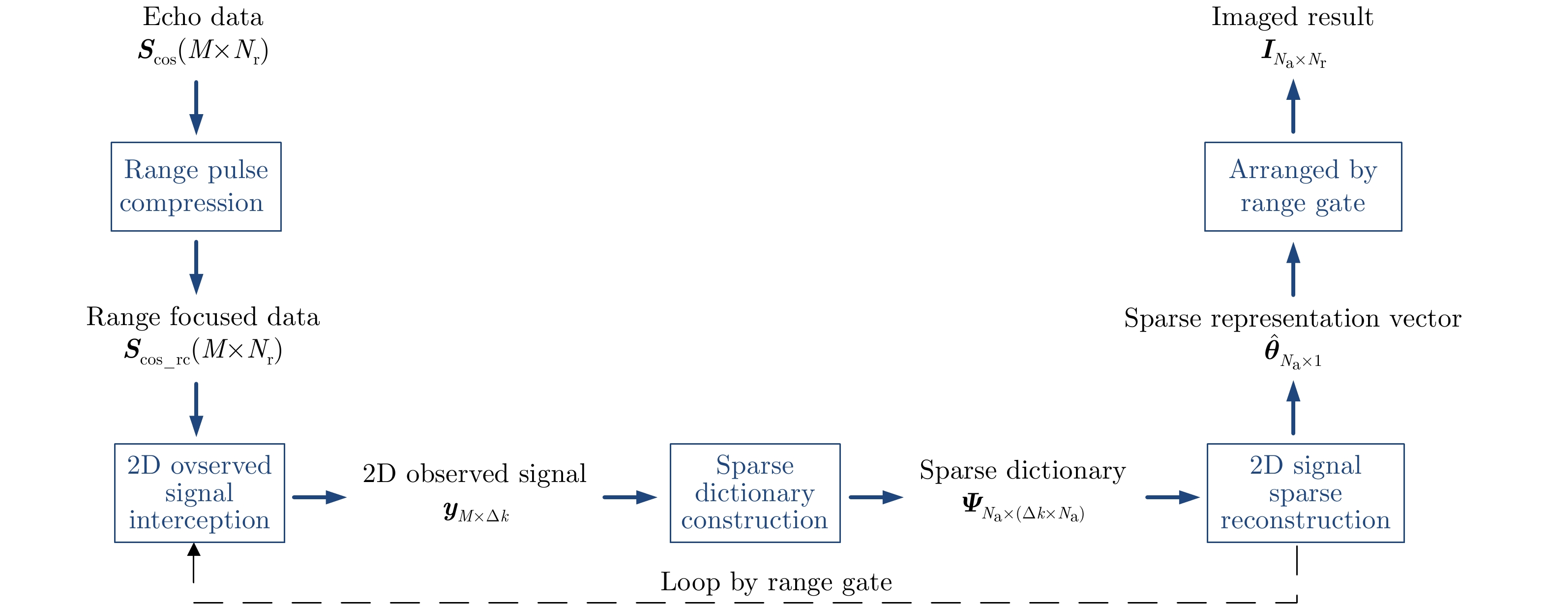
Co-prime-sampling space-borne Synthetic Aperture Radar (SAR) replaces the traditional uniform sampling by performing co-prime sampling in azimuth, which effectively alleviates the conflict between spatial resolution and effective swath width, while also improving the ground detection performance of the SAR system. However, co-prime-sampling in azimuth causes the echo signal to exhibit azimuthal under sampling and non-uniform sampling characteristics, which means the traditional SAR image-processing method can not effectively image co-prime-sampled SAR. In this paper, an imaging method based on Two-Dimensional (2D) sparse-signal reconstruction is proposed for co-prime-sampling space-borne SAR. Using this method, after range-pulse compression, the 2D observed signal is intercepted and a corresponding sparse dictionary consisting of 2D atoms is constructed according to the Doppler parameters of each range gate. Then, azimuth-focus processing is completed by the improved 2D-signal sparsity adaptive matching pursuit algorithm. The proposed method not only compensates for the 2D coupling between the range and azimuth, but also eliminates the influence of space-varying imaging parameters on sparse reconstruction to achieve accurate reconstruction of the entire scene. The simulation results of the point targets and distribution targets verify that the proposed method can effectively reconstruct sparse scenes at a rate much lower than the Nyquist sampling rate. -

-
References
[1] 李春升, 杨威, 王鹏波. 星载SAR成像处理算法综述[J]. 雷达学报, 2013, 2(1): 111–122. doi: 10.3724/SP.J.1300.2013.20071LI Chunsheng, YANG Wei, and WANG Pengbo. A review of spaceborne SAR algorithm for image formation[J]. Journal of Radars, 2013, 2(1): 111–122. doi: 10.3724/SP.J.1300.2013.20071[2] 邓云凯, 赵凤军, 王宇. 星载SAR技术的发展趋势及应用浅析[J]. 雷达学报, 2012, 1(1): 1–10. doi: 10.3724/SP.J.1300.2012.20015DENG Yunkai, ZHAO Fengjun, and WANG Yu. Brief analysis on the development and application of spaceborne SAR[J]. Journal of Radars, 2012, 1(1): 1–10. doi: 10.3724/SP.J.1300.2012.20015[3] 赵耀, 邓云凯, 王宇, 等. 原始数据压缩对方位向多通道SAR系统影响研究[J]. 雷达学报, 2017, 6(4): 397–407. doi: 10.12000/JR17030ZHAO Yao, DENG Yunkai, WANG Yu, et al. Study of effect of raw data compression on azimuth multi-channel SAR system[J]. Journal of Radars, 2017, 6(4): 397–407. doi: 10.12000/JR17030[4] 罗绣莲, 徐伟, 郭磊. 捷变PRF技术在斜视聚束SAR中的应用[J]. 雷达学报, 2015, 4(1): 70–77. doi: 10.12000/JR14149LUO Xiulian, XU Wei, and GUO Lei. The application of PRF variation to squint spotlight SAR[J]. Journal of Radars, 2015, 4(1): 70–77. doi: 10.12000/JR14149[5] DONOHO D L. Compressed sensing[J]. IEEE Transactions on Information Theory, 2006, 52(4): 1289–1306. doi: 10.1109/TIT.2006.871582[6] ENDER J H G. On compressive sensing applied to radar[J]. Signal Processing, 2010, 90(5): 1402–1414. doi: 10.1016/j.sigpro.2009.11.009[7] VAIDYANATHAN P P and PAL P. Sparse sensing with co-prime samplers and arrays[J]. IEEE Transactions on Signal Processing, 2011, 59(2): 573–586. doi: 10.1109/TSP.2010.2089682[8] VAIDYANATHAN P P and PAL P. Theory of sparse coprime sensing in multiple dimensions[J]. IEEE Transactions on Signal Processing, 2011, 59(8): 3592–3608. doi: 10.1109/tsp.2011.2135348[9] ZHANG Y D, AMIN M G, and HIMED B. Sparsity-based DOA estimation using co-prime arrays[C]. 2013 IEEE International Conference on Acoustics, Speech and Signal Processing, Vancouver, Canada, 2013. doi: 10.1109/ICASSP.2013.6638403.[10] TAN Zhao, ELDAR Y C, and NEHORAI A. Direction of arrival estimation using co-prime arrays: A super resolution viewpoint[J]. IEEE Transactions on Signal Processing, 2014, 62(21): 5565–5576. doi: 10.1109/TSP.2014.2354316[11] YU Lei, WEI Yinsheng, and LIU Wei. Adaptive beamforming based on nonuniform linear arrays with enhanced degrees of freedom[C]. TENCON 2015- 2015 IEEE Region 10 Conference, Macao, China, 2015. doi: 10.1109/TENCON.2015.7373099.[12] QIN Si, ZHANG Y D, and AMIN M G. Generalized coprime array configurations for direction-of-arrival estimation[J]. IEEE Transactions on Signal Processing, 2015, 63(6): 1377–1390. doi: 10.1109/TSP.2015.2393838[13] SUN Fenggang, GAO Bin, CHEN Lizhen, et al. A low-complexity ESPRIT-based DOA estimation method for co-prime linear arrays[J]. Sensors, 2016, 16(9): 1367. doi: 10.3390/s16091367[14] 王龙刚, 李廉林. 基于互质阵列雷达技术的近距离目标探测方法(英文)[J]. 雷达学报, 2016, 5(3): 244–253. doi: 10.12000/JR16022WANG Longgang and LI Lianlin. Short-range radar detection with (M, N)-coprime array configurations[J]. Journal of Radars, 2016, 5(3): 244–253. doi: 10.12000/JR16022[15] SUN Fenggang, LAN Peng, and ZHANG Guowei. Reduced dimension based two-dimensional DOA estimation with full DOFs for generalized co-prime planar arrays[J]. Sensors, 2018, 18(6): 1725. doi: 10.3390/s18061725[16] RAZA A, LIU Wei, and SHEN Qing. Thinned coprime array for second-order difference co-array generation with reduced mutual coupling[J]. IEEE Transactions on Signal Processing, 2019, 67(8): 2052–2065. doi: 10.1109/TSP.2019.2901380[17] DI MARTINO G and IODICE A. Orthogonal coprime synthetic aperture radar[J]. IEEE Transactions on Geoscience and Remote Sensing, 2017, 55(1): 432–440. doi: 10.1109/TGRS.2016.2608140[18] TAO Yu, ZHANG Gong, and LI Daren. Coprime sampling with deterministic digital filters in compressive sensing radar[C]. 2016 CIE International Conference on Radar, Guangzhou, China, 2016. doi: 10.1109/RADAR.2016.8059224.[19] SHI Hongyin and JIA Baojing. SAR imaging method based on coprime sampling and nested sparse sampling[J]. Journal of Systems Engineering and Electronics, 2015, 26(6): 1222–1228. doi: 10.1109/JSEE.2015.00134[20] CAFFORIO C, PRATI C, and ROCCA F. SAR data focusing using seismic migration techniques[J]. IEEE Transactions on Aerospace and Electronic Systems, 1991, 27(2): 194–207. doi: 10.1109/7.78293[21] MITTERMAYER J, MOREIRA A, and LOFFELD O. Spotlight SAR data processing using the frequency scaling algorithm[J]. IEEE Transactions on Geoscience and Remote Sensing, 1999, 37(5): 2198–2214. doi: 10.1109/36.789617[22] SUN Xiaobing, YEO T S, and ZHANG Chengbo, et al. Time-varying step-transform algorithm for high squint SAR imaging[J]. IEEE Transactions on Geoscience and Remote Sensing, 1999, 37(6): 2668–2677. doi: 10.1109/36.803414[23] WANG Pengbo, LIU Wei, CHEN Jie, et al. A high-order imaging algorithm for high-resolution spaceborne SAR based on a modified equivalent squint range model[J]. IEEE Transactions on Geoscience and Remote Sensing, 2015, 53(3): 1225–1235. doi: 10.1109/TGRS.2014.2336241[24] DO T T, GAN Lu, NGUYEN N, et al. Sparsity adaptive matching pursuit algorithm for practical compressed sensing[C]. The 42nd Asilomar Conference on Signals, Systems and Computers, Pacific Grove, 2008. doi: 10.1109/ACSSC.2008.5074472. -
Proportional views

- Publishing Ethics
- Journal Insights
- Abstracting & Indexing
- Peer Review Policies
- Guide for Authors
- Conference
- ISSN 2095-283X (Print)ISSN 2097-339X (Online)
- CN 10-1030/TN
- CODEN LXEUAO
About Journal
- Sponsor: China Radio Detection and Ranging Industry Association (CRIA)
- Phone: 010-58887062
- Email:radars@aircas.ac.cn
- Publisher: Leida Xuebao Bianjibu (Editorial office of the Journal of Radars)
Contacts Us

京ICP备20021838号-14
Supported by: Beijing Renhe Information Technology Co. Ltd

Export File
Citation
Format
Content
 DownLoad:


- Figure 1. Structure of an (M, N)-co-prime array
- Figure 2. Schematic diagram of co-prime-sampling spaceborne SAR
- Figure 3. Geometry of a typical space-borne SAR
- Figure 4. A 2-D observed signal is intercepted form the range-focused signal
- Figure 5. General flow chart of the imaging method based on 2D sparse signal reconstruction for co-prime-sampling spaceborne SAR
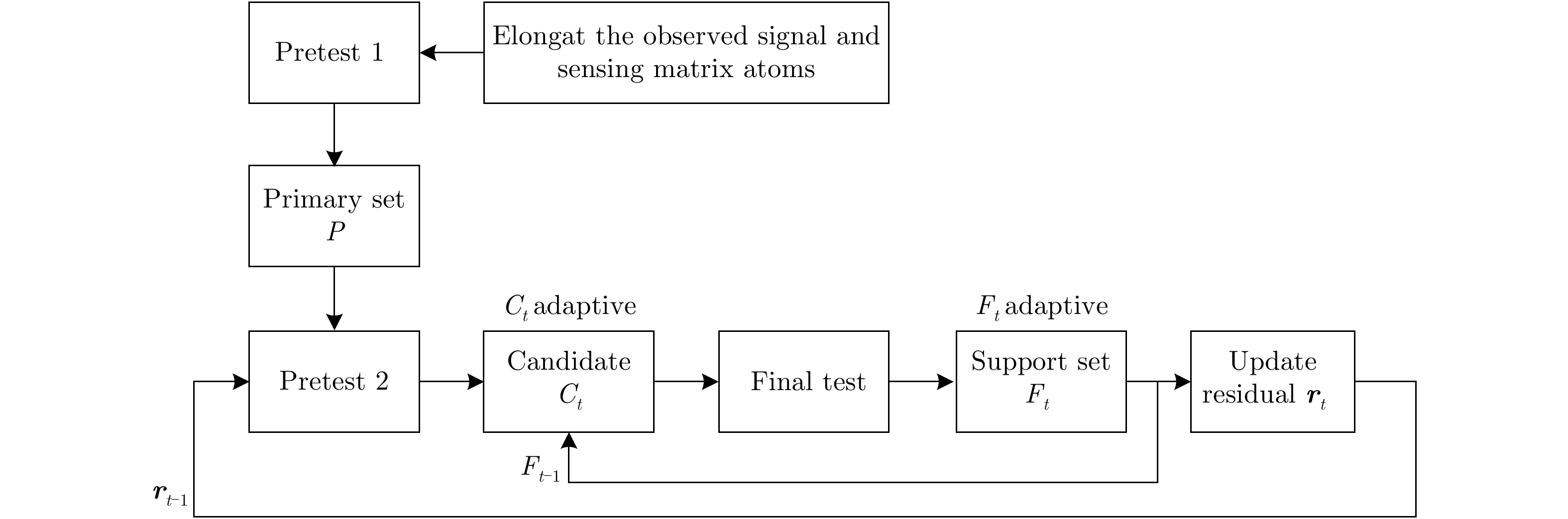
- Figure 6. Block diagram of the improved 2D SAMP algorithm
- Figure 7. A sensing matrix containing atoms with the same effective echo position.
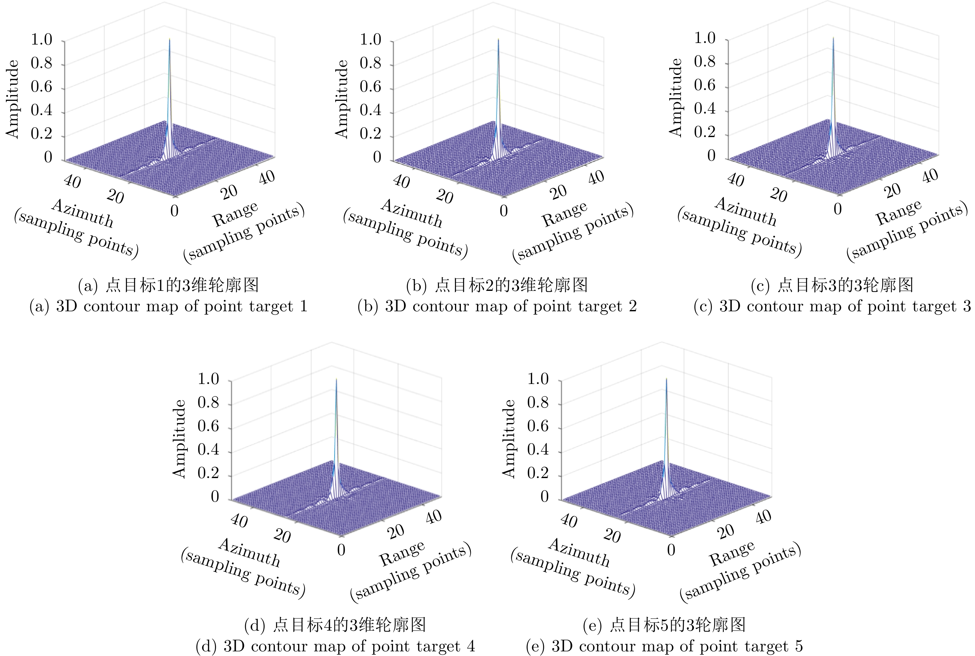
- Figure 8. Reconstruction results of point targets
- Figure 9. 3D contour map of each point target
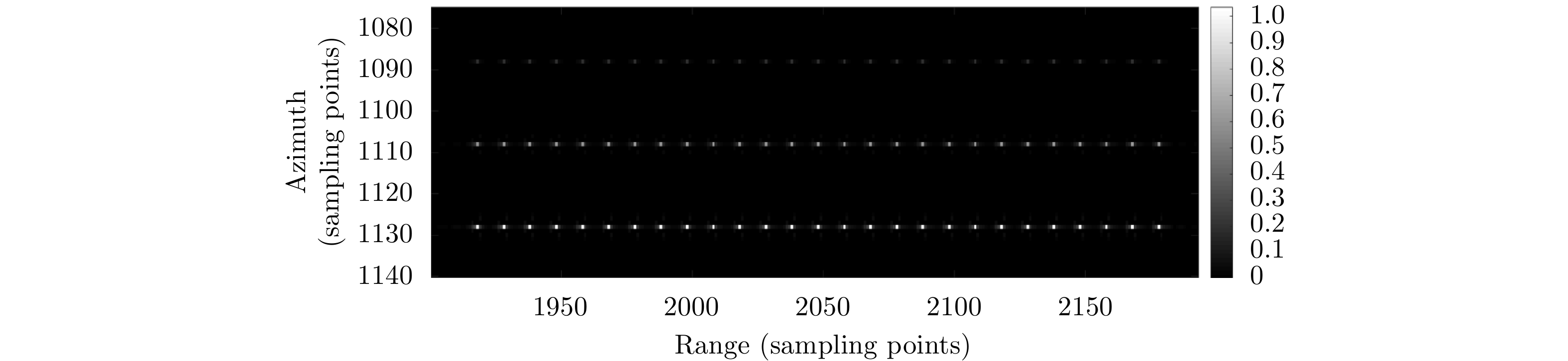
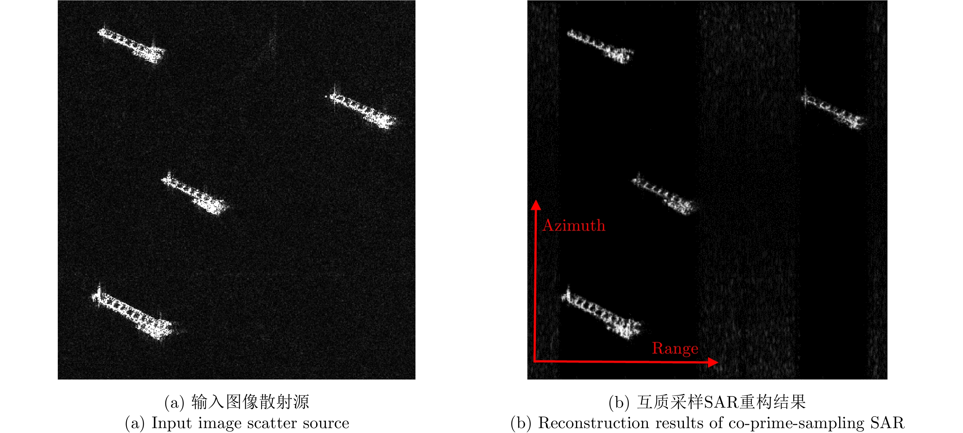
- Figure 10. Reconstruction results of multiple point targets
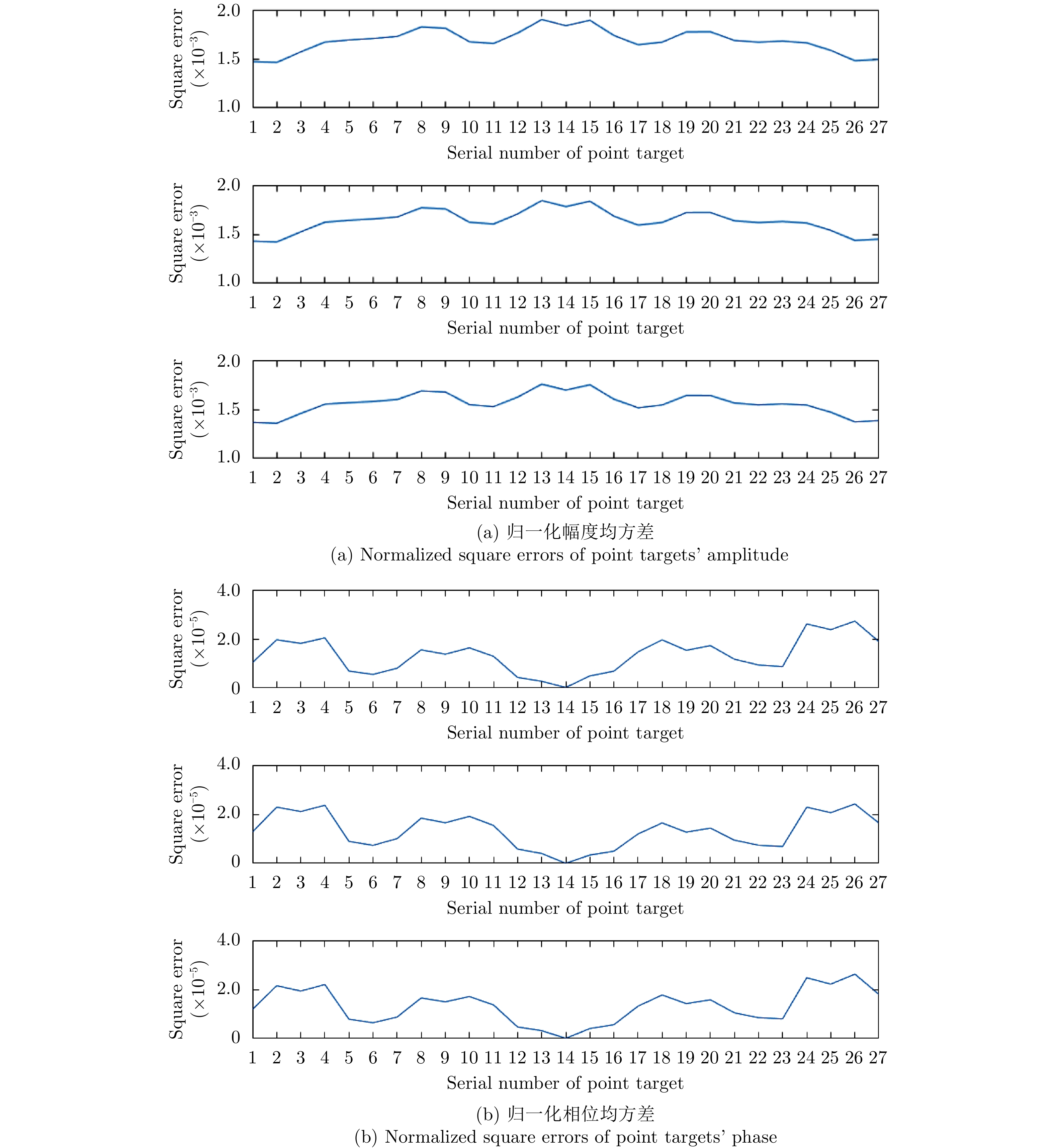
- Figure 11. The amplitude error curve and phase error curve of the point targets in the reconstruction result
- Figure 12. TerraSAR-X Level1 SSC product image
- Figure 13. Sea surface target imaging simulation result