
 Submit Manuscript
 Peer Review
 Editor Work
- Home
- Articles & Issues
-
Data
- Dataset of Radar Detecting Sea
- SAR Dataset
- SARGroundObjectsTypes
- SARMV3D
- AIRSAT Constellation SAR Land Cover Classification Dataset
- 3DRIED
- UWB-HA4D
- LLS-LFMCWR
- FAIR-CSAR
- MSAR
- SDD-SAR
- FUSAR
- SpaceborneSAR3Dimaging
- Sea-land Segmentation
- SAR Multi-domain Ship Detection Dataset
- SAR-Airport
- Hilly and mountainous farmland time-series SAR and ground quadrat dataset
- SAR images for interference detection and suppression
- HP-SAR Evaluation & Analytical Dataset
- GDHuiYan-ATRNet
- Multi-System Maritime Low Observable Target Dataset
- DatasetinthePaper
- DatasetintheCompetition
- Report
- Course
- About
- Publish
- Editorial Board
- Chinese
| Citation: | LENG Xiangguang, JI Kefeng, XIONG Boli, et al. Statistical modeling methods of single-channel complex-valued SAR images for ship detection
[J]. Journal of Radars, 2020, 9(3): 477–496. doi: 10.12000/JR20070

|
Statistical Modeling Methods of Single-channel Complex-valued SAR Images for Ship Detection
DOI: 10.12000/JR20070 CSTR: 32380.14.JR20070
More Information-
Abstract
Synthetic Aperture Radar (SAR), which features rich imaging modes, wide coverage, and high resolution, is an effective technique for long-term, dynamic, and large-scale monitoring of the ocean. Under the assumption of fully developed speckle, traditional ship detection methods in single-channel SAR images focus mainly on amplitude information. Since conventional assumptions are not strictly true in high-resolution situations, this prevents the full investigation of phase or complex-valued information in single-channel SAR images. In this paper, with a focus on ship detection applications, we categories the methods used in the statistical modeling of single-channel complex-valued SAR images as amplitude-, phase-, or complex-valued-based. After providing a brief overview of amplitude statistical modeling methods, we focus on phase and complex-valued statistical modeling methods of single-channel SAR images, describing their modeling processes and parameter estimation methods. We then present the results of our recent ship detection research based on complex-valued statistical information in single-channel SAR images and make suggestions regarding future research. -

-
References
[1] LEE J S and POTTIER E. Polarimetric Radar Imaging: From Basics to Applications[M]. Boca Raton: CRC Press, 2009.[2] OLIVER C and QUEGAN S. Understanding Synthetic Aperture Radar Images[M]. Boston: SciTech Publishing, 2004.[3] 邓云凯, 赵凤军, 王宇. 星载SAR技术的发展趋势及应用浅析[J]. 雷达学报, 2012, 1(1): 1–10. doi: 10.3724/SP.J.1300.2012.20015DENG Yunkai, ZHAO Fengjun, and WANG Yu. Brief analysis on the development and application of Spaceborne SAR[J]. Journal of Radars, 2012, 1(1): 1–10. doi: 10.3724/SP.J.1300.2012.20015[4] 杨建宇. 雷达对地成像技术多向演化趋势与规律分析[J]. 雷达学报, 2019, 8(6): 669–692. doi: 10.12000/JR19099YANG Jianyu. Multi-directional evolution trend and law analysis of radar ground imaging technology[J]. Journal of Radars, 2019, 8(6): 669–692. doi: 10.12000/JR19099[5] 金亚秋. 多模式遥感智能信息与目标识别: 微波视觉的物理智能[J]. 雷达学报, 2019, 8(6): 710–716. doi: 10.12000/JR19083JIN Yaqiu. Multimode remote sensing intelligent information and target recognition: Physical intelligence of microwave vision[J]. Journal of Radars, 2019, 8(6): 710–716. doi: 10.12000/JR19083[6] 杜兰, 王兆成, 王燕, 等. 复杂场景下单通道SAR目标检测及鉴别研究进展综述[J]. 雷达学报, 2020, 9(1): 34–54. doi: 10.12000/JR19104DU Lan, WANG Zhaocheng, WANG Yan, et al. Survey of research progress on target detection and discrimination of single-channel SAR images for complex scenes[J]. Journal of Radars, 2020, 9(1): 34–54. doi: 10.12000/JR19104[7] CRISP D J. The state-of-the-art in ship detection in synthetic aperture radar imagery[R]. DATO-RR-0272, 2004.[8] GAO G, GAO S, and HE J. Maritime Surveillance with SAR Data[M]. Chapter. Ship Detection. IET book, in publishing.[9] GAO Gui. Statistical modeling of SAR images: A survey[J]. Sensors, 2010, 10(1): 775–795. doi: 10.3390/s100100775[10] VESPE M and GREIDANUS H. SAR image quality assessment and indicators for vessel and oil spill detection[J]. IEEE Transactions on Geoscience and Remote Sensing, 2012, 50(11): 4726–4734. doi: 10.1109/TGRS.2012.2190293[11] VELOTTO D, SOCCORSI M, and LEHNER S. Azimuth ambiguities removal for ship detection using full polarimetric X-band SAR data[J]. IEEE Transactions on Geoscience and Remote Sensing, 2014, 52(1): 76–88. doi: 10.1109/TGRS.2012.2236337[12] GREIDANUS H, CLAYTON P, INDREGARD M, et al. Benchmarking operational SAR ship detection[C]. 2004 IEEE International Geoscience and Remote Sensing Symposium, Anchorage, USA, 2004: 4215–4218.[13] OUCHI K. Current status on vessel detection and classification by synthetic aperture radar for maritime security and safety[C]. The 38th Symposium on Remote Sensing for Environmental Sciences, Gamagori, Aichi, Japan, 2016: 5–12.[14] PAN Zongxu, LIU Lei, QIU Xiaolan, et al. Fast vessel detection in Gaofen-3 SAR images with ultrafine strip-map mode[J]. Sensors, 2017, 17(7): 1578. doi: 10.3390/s17071578[15] AN Quanzhi, PAN Zongxu, and YOU Hongjian. Ship detection in Gaofen-3 SAR images based on sea clutter distribution analysis and deep convolutional neural network[J]. Sensors, 2018, 18(2): 334. doi: 10.3390/s18020334[16] WANG Shigang, WANG Min, YANG Shuyuan, et al. New hierarchical saliency filtering for fast ship detection in high-resolution SAR images[J]. IEEE Transactions on Geoscience and Remote Sensing, 2017, 55(1): 351–362. doi: 10.1109/TGRS.2016.2606481[17] IERVOLINO P and GUIDA R. A novel ship detector based on the generalized-likelihood ratio test for SAR imagery[J]. IEEE Journal of Selected Topics in Applied Earth Observations and Remote Sensing, 2017, 10(8): 3616–3630. doi: 10.1109/JSTARS.2017.2692820[18] LENG Xiangguang, JI Kefeng, YANG Kai, et al. A bilateral CFAR algorithm for ship detection in SAR images[J]. IEEE Geoscience and Remote Sensing Letters, 2015, 12(7): 1536–1540. doi: 10.1109/LGRS.2015.2412174[19] LENG Xiangguang, JI Kefeng, ZHOU Shilin, et al. An adaptive ship detection scheme for spaceborne SAR imagery[J]. Sensors, 2016, 16(9): 1345. doi: 10.3390/s16091345[20] LENG Xiangguang, JI Kefeng, XING Xiangwei, et al. Area ratio invariant feature group for ship detection in SAR imagery[J]. IEEE Journal of Selected Topics in Applied Earth Observations and Remote Sensing, 2018, 11(7): 2376–2388. doi: 10.1109/JSTARS.2018.2820078[21] LENG Xiangguang, JI Kefeng, ZHOU Shilin, et al. Ship detection based on complex signal kurtosis in single-channel SAR imagery[J]. IEEE Transactions on Geoscience and Remote Sensing, 2019, 57(9): 6447–6461. doi: 10.1109/TGRS.2019.2906054[22] LENG Xiangguang, JI Kefeng, ZHOU Shilin, et al. Discriminating ship from radio frequency interference based on noncircularity and non-Gaussianity in Sentinel-1 SAR imagery[J]. IEEE Transactions on Geoscience and Remote Sensing, 2019, 57(1): 352–363. doi: 10.1109/TGRS.2018.2854661[23] EL-DARYMLI K, MCGUIRE P, GILL E W, et al. Characterization and statistical modeling of phase in single-channel synthetic aperture radar imagery[J]. IEEE Transactions on Aerospace and Electronic Systems, 2015, 51(3): 2071–2092. doi: 10.1109/TAES.2015.140711[24] EL-DARYMLI K, MOLONEY C, GILL E, et al. Nonlinearity and the effect of detection on single-channel synthetic aperture radar imagery[C]. OCEANS 2014-TAIPEI, Taipei, China, 2014: 1–7.[25] OLLILA E. On the circularity of a complex random variable[J]. IEEE Signal Processing Letters, 2008, 15: 841–844. doi: 10.1109/LSP.2008.2005050[26] OLLILA E, KOIVUNEN V, and POOR H V. Complex-valued signal processing—essential models, tools and statistics[C]. 2011 Information Theory and Applications Workshop, La Jolla, USA, 2011: 1–10.[27] OLLILA E, ERIKSSON J, and KOIVUNEN V. Complex elliptically symmetric random variables—Generation, characterization, and circularity tests[J]. IEEE Transactions on Signal Processing, 2011, 59(1): 58–69. doi: 10.1109/TSP.2010.2083655[28] ERIKSSON J and KOIVUNEN V. Complex random vectors and ICA models: Identifiability, uniqueness, and separability[J]. IEEE Transactions on Information Theory, 2006, 52(3): 1017–1029. doi: 10.1109/TIT.2005.864440[29] ERIKSSON J, OLLILA E, and KOIVUNEN V. Essential statistics and tools for complex random variables[J]. IEEE Transactions on Signal Processing, 2010, 58(10): 5400–5408. doi: 10.1109/TSP.2010.2054085[30] NOVEY M, ADALI T, and ROY A. Circularity and Gaussianity detection using the complex generalized Gaussian distribution[J]. IEEE Signal Processing Letters, 2009, 16(11): 993–996. doi: 10.1109/LSP.2009.2028412[31] NOVEY M, ADALI T, and ROY A. A complex generalized Gaussian distribution—Characterization, generation, and estimation[J]. IEEE Transactions on Signal Processing, 2010, 58(3): 1427–1433. doi: 10.1109/TSP.2009.2036049[32] NOVEY M, OLLILA E, and ADALI T. On testing the extent of noncircularity[J]. IEEE Transactions on Signal Processing, 2011, 59(11): 5632–5637. doi: 10.1109/TSP.2011.2162951[33] SCHREIER P J and SCHARF L L. Statistical Signal Processing of Complex-valued Data: The Theory of Improper and Noncircular Signals[M]. Cambridge: Cambridge University Press, 2010.[34] WU Wenjin, GUO Huadong, LI Xinwu, et al. Urban land use information extraction using the ultrahigh-resolution Chinese airborne SAR imagery[J]. IEEE Transactions on Geoscience and Remote Sensing, 2015, 53(10): 5583–5599. doi: 10.1109/TGRS.2015.2425658[35] WU Wenjin, LI Xinwu, GUO Huadong, et al. Noncircularity parameters and their potential applications in UHR MMW SAR data sets[J]. IEEE Geoscience and Remote Sensing Letters, 2016, 13(10): 1547–1551. doi: 10.1109/LGRS.2016.2595762[36] SOCCORSI M and DATCU M. Stochastic models of SLC HR SAR images[C]. 2007 IEEE International Geoscience and Remote Sensing Symposium, Barcelona, Spain, 2007: 3887–3890.[37] SOCCORSI M, DATCU M, and GLEICH D. TerraSAR-X: Complex Image Inversion for Feature Extraction[C]. 2008 IEEE International Geoscience and Remote Sensing Symposium, Boston, USA, 2008: III-99–III-102.[38] 冷祥光, 计科峰, 周石琳. SAR图像方位模糊去除方法研究[C]. 第五届高分辨率对地观测学术年会论文集, 西安, 2018.LENG Xiangguang, JI Kefeng, and ZHOU Shilin. Research on azimuth ambiguity removal methods in SAR imagery[C]. The 5th China High Resolution Earth Observation Conference, Xi’an, China, 2018.[39] LENG Xiangguang, JI Kefeng, ZHOU Shilin, et al. Azimuth ambiguities removal in littoral zones based on multi-temporal SAR images[J]. Remote Sensing, 2017, 9(8): 866. doi: 10.3390/rs9080866[40] JAKEMAN E and PUSEY P. A model for non-Rayleigh sea echo[J]. IEEE Transactions on Antennas and Propagation, 1976, 24(6): 806–814. doi: 10.1109/TAP.1976.1141451[41] GOLDSTEIN G B. False-alarm regulation in log-normal and Weibull clutter[J]. IEEE Transactions on Aerospace and Electronic Systems, 1973, AES–9(1): 84–92.[42] TRUNK G V and GEORGE S F. Detection of targets in non-Gaussian sea clutter[J]. IEEE Transactions on Aerospace and Electronic Systems, 1970, AES–6(5): 620–628.[43] DANA R A and KNEPP D L. The impact of strong scintillation on space based radar design II: Noncoherent detection[J]. IEEE Transactions on Aerospace and Electronic Systems, 1986, AES–22(1): 34–46.[44] TISON C, NICOLAS J M, TUPIN F, et al. A new statistical model for Markovian classification of urban areas in high-resolution SAR images[J]. IEEE Transactions on Geoscience and Remote Sensing, 2004, 42(10): 2046–2057. doi: 10.1109/TGRS.2004.834630[45] KURUOGLU E E and ZERUBIA J. Modeling SAR images with a generalization of the Rayleigh distribution[J]. IEEE Transactions on Image Processing, 2004, 13(4): 527–533. doi: 10.1109/TIP.2003.818017[46] MIGLIACCIO M, FERRARA G, GAMBARDELLA A, et al. A physically consistent speckle model for marine SLC SAR images[J]. IEEE Journal of Oceanic Engineering, 2007, 32(4): 839–847. doi: 10.1109/JOE.2007.903985[47] LIAO Mingsheng, WANG Changcheng, WANG Yong, et al. Using SAR images to detect ships from sea clutter[J]. IEEE Geoscience and Remote Sensing Letters, 2008, 5(2): 194–198. doi: 10.1109/LGRS.2008.915593[48] FERRARA G, MIGLIACCIO M, NUNZIATA F, et al. Generalized-K (GK)-based observation of metallic objects at sea in full-resolution Synthetic Aperture Radar (SAR) data: A multipolarization study[J]. IEEE Journal of Oceanic Engineering, 2011, 36(2): 195–204. doi: 10.1109/JOE.2011.2109491[49] SAHED M, MEZACHE A, and LAROUSSI T. A novel [z log(z)]-based closed form approach to parameter estimation of K-distributed clutter plus noise for radar detection[J]. IEEE Transactions on Aerospace and Electronic Systems, 2015, 51(1): 492–505. doi: 10.1109/TAES.2014.140180[50] ROSENBERG L, WATTS S, and BOCQUET S. Application of the K+Rayleigh distribution to high grazing angle sea-clutter[C]. 2014 International Radar Conference, Lille, France, 2014: 1–6.[51] ROSENBERG L and BOCQUET S. Application of the Pareto plus noise distribution to medium grazing angle sea-clutter[J]. IEEE Journal of Selected Topics in Applied Earth Observations and Remote Sensing, 2015, 8(1): 255–261. doi: 10.1109/JSTARS.2014.2347957[52] MIDDLETON D. New physical-statistical methods and models for clutter and reverberation: The KA-distribution and related probability structures[J]. IEEE Journal of Oceanic Engineering, 1999, 24(3): 261–284. doi: 10.1109/48.775289[53] DONG Yunhan. Distribution of X-band high resolution and high grazing angle sea clutter[R]. DSTO-RR-0316, 2006.[54] ROSENBERG L, CRISP D J, and STACY N J. Analysis of the KK-distribution with medium grazing angle sea-clutter[J]. IET Radar, Sonar & Navigation, 2010, 4(2): 209–222.[55] FICHE A, ANGELLIAUME S, ROSENBERG L, et al. Analysis of X-band SAR sea-clutter distributions at different grazing angles[J]. IEEE Transactions on Geoscience and Remote Sensing, 2015, 53(8): 4650–4660. doi: 10.1109/TGRS.2015.2405577[56] FICHE A, ANGELLIAUME S, ROSENBERG L, et al. Statistical analysis of low grazing angle high resolution X-band SAR sea clutter[C]. 2014 International Radar Conference, Lille, France, 2014: 1–6.[57] 秦先祥. 基于广义Gamma分布的SAR图像统计建模及应用研究[D]. [博士论文], 国防科学技术大学, 2015.QIN Xianxiang. Research on statistical modeling of SAR images and its application based on generalized Gamma distribution[D]. [Ph. D. Dissertation], National University of Defense Technology, 2015.[58] ACHIM A, KURUOGLU E E, and ZERUBIA J. SAR image filtering based on the heavy-tailed Rayleigh model[J]. IEEE Transactions on Image Processing, 2006, 15(9): 2686–2693. doi: 10.1109/TIP.2006.877362[59] RIHACZEK A W and HERSHKOWITZ S J. Theory and Practice of Radar Target Identification[M]. Boston: Artech House, 2000.[60] RIHACZEK A W and HERSHKOWITZ S J. Radar Resolution and Complex-image Analysis[M]. Boston: Artech House, 1996.[61] JAO J K, LEE C E, and AYASLI S. Coherent spatial filtering for SAR detection of stationary targets[J]. IEEE Transactions on Aerospace and Electronic systems, 1999, 35(2): 614–626. doi: 10.1109/7.766942[62] DATCU M, SCHWARZ G, SOCCORSI M, et al. Phase information contained in meter-scale SAR images[C]. SPIE SAR Image Analysis, Modeling, and Techniques IX, Florence, Italy, 2007: 67460H.[63] Circular data analysis[EB/OL]. https://ncss-wpengine.netdna-ssl.com/wp-content/themes/ncss/pdf/Procedures/NCSS/Circular_Data_Analysis.pdf.[64] FISHER N I. Statistical Analysis of Circular Data[M]. Cambridge: Cambridge University Press, 1995.[65] MARDIA K V and JUPP P E. Directional Statistics[M]. Chichester: John Wiley & Sons, 2009.[66] EVANS M, HASTINGS N, and PEACOCK B. Statistical Distributions[M]. 3rd ed. New York: Wiley, 2000: 117–118.[67] EL-DARYMLI K, MCGUIRE P, POWER D, et al. Rethinking the phase in single-channel SAR imagery[C]. 2013 14th International Radar Symposium, Dresden, Germany, 2013: 429–436.[68] EL-DARYMLI K, MOLONEY C, GILL E, et al. On circularity/noncircularity in single-channel synthetic aperture radar imagery[C]. 2014 Oceans-St. John’s, St. John’s, Canada, 2014: 1–4.[69] EL-DARYMLI K, MCGUIRE P, GILL E W, et al. Holism-based features for target classification in focused and complex-valued synthetic aperture radar imagery[J]. IEEE Transactions on Aerospace and Electronic Systems, 2016, 52(2): 786–808. doi: 10.1109/TAES.2015.140757[70] LENG Xiangguang, JI Kefeng, ZHOU Shilin, et al. Fast shape parameter estimation of the complex generalized Gaussian distribution in SAR images[J]. IEEE Geoscience and Remote Sensing Letters, 2020, in press. doi: 10.1109/LGRS.2019.2960095[71] FANG Kaitai, KOTZ S, and NG K W. Symmetric Multivariate and Related Distributions[M]. London: Chapman and Hall, 1990.[72] LI Hualiang and ADALI T. A class of complex ICA algorithms based on the kurtosis cost function[J]. IEEE Transactions on Neural Networks, 2008, 19(3): 408–420. doi: 10.1109/TNN.2007.908636[73] DOUGLAS S C. Fixed-point algorithms for the blind separation of arbitrary complex-valued non-Gaussian signal mixtures[J]. EURASIP Journal on Advances in Signal Processing, 2007, 2007: 036525. doi: 10.1155/2007/36525[74] LENG X. Fast shape parameter estimation method for CGGD[EB/OL]. https://www.mathworks.com/matlabcentral/fileexchange/69582-shape-paramter-estimation-implementation-for-the-cggd, 2018.[75] LENG Xiangguang, JI Kefeng, and ZHOU Shilin. A novel ship segmentation method based on kurtosis test in complex-valued SAR imagery[C]. 2018 10th IAPR Workshop on Pattern Recognition in Remote Sensing, Beijing, China, 2018: 1–4.[76] LENG X. Opensarshipfilter-package-sourcecode[EB/OL]. https://www.mathworks.com/matlabcentral/fileexchange/66929-opensarshipfilter-package-sourcecode, 2018.[77] Shanghai Jiaotong University. Opensar platform[EB/OL]. http://opensar.sjtu.edu.cn/, 2017.[78] HUANG Lanqing, LIU Bin, LI Boying, et al. OpenSARShip: A dataset dedicated to Sentinel-1 ship interpretation[J]. IEEE Journal of Selected Topics in Applied Earth Observations and Remote Sensing, 2018, 11(1): 195–208. doi: 10.1109/JSTARS.2017.2755672[79] SANTAMARIA C, ALVAREZ M, GREIDANUS H, et al. Mass processing of Sentinel-1 images for maritime surveillance[J]. Remote Sensing, 2017, 9(7): 678. doi: 10.3390/rs9070678[80] MANSOUR A and JUTTEN C. What should we say about the kurtosis?[J]. IEEE Signal Processing Letters, 1999, 6(12): 321–322. doi: 10.1109/97.803435[81] DUMITRU O C and DATCU M. Information content of very high resolution SAR images: Study of dependency of SAR image structure descriptors with incidence angle[J]. International Journal on Advances in Telecommunications, 2012, 5(3/4): 239–251. -
Proportional views

- Publishing Ethics
- Journal Insights
- Abstracting & Indexing
- Peer Review Policies
- Guide for Authors
- Conference
- ISSN 2095-283X (Print)ISSN 2097-339X (Online)
- CN 10-1030/TN
- CODEN LXEUAO
About Journal
- Sponsor: China Radio Detection and Ranging Industry Association (CRIA)
- Phone: 010-58887062
- Email:radars@aircas.ac.cn
- Publisher: Leida Xuebao Bianjibu (Editorial office of the Journal of Radars)
Contacts Us

京ICP备20021838号-14
Supported by: Beijing Renhe Information Technology Co. Ltd

Export File
Citation
Format
Content
 DownLoad:


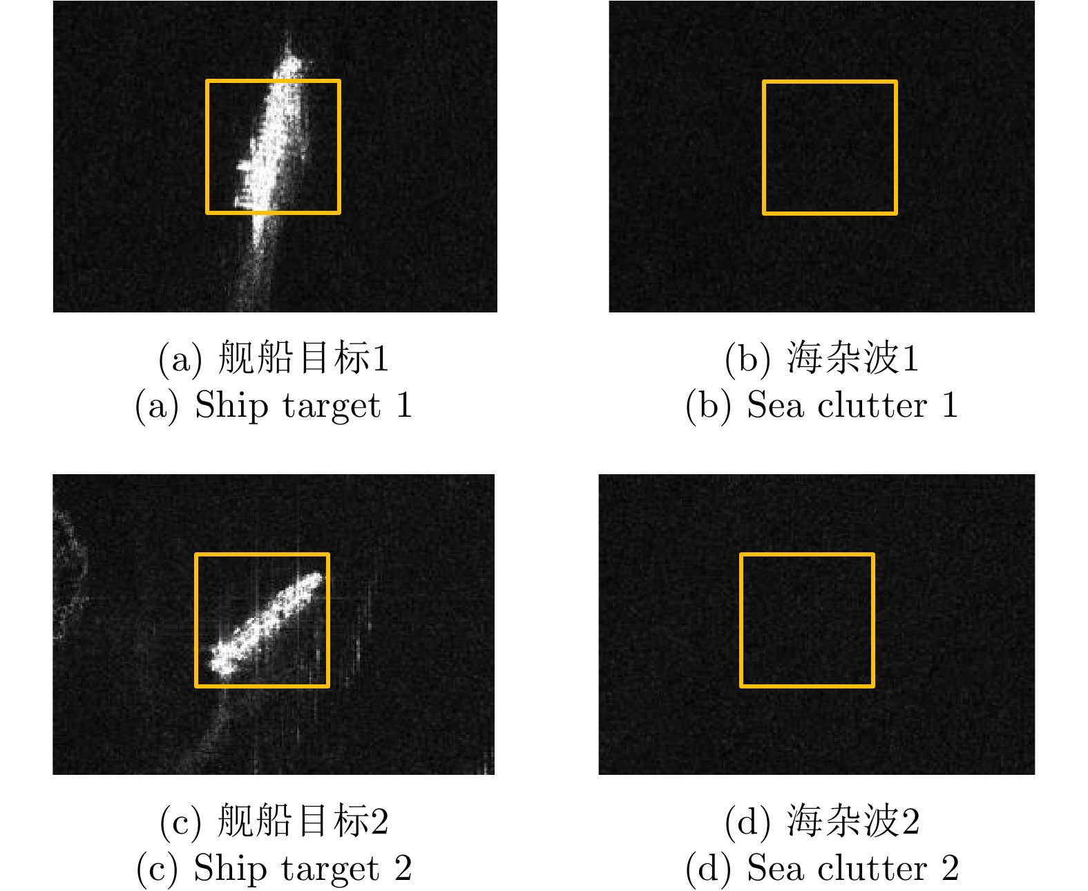
- Figure 1. TerraSAR-X ship target and sea clutter amplitude images
- Figure 2. TerraSAR-X ship target and sea clutter phase images
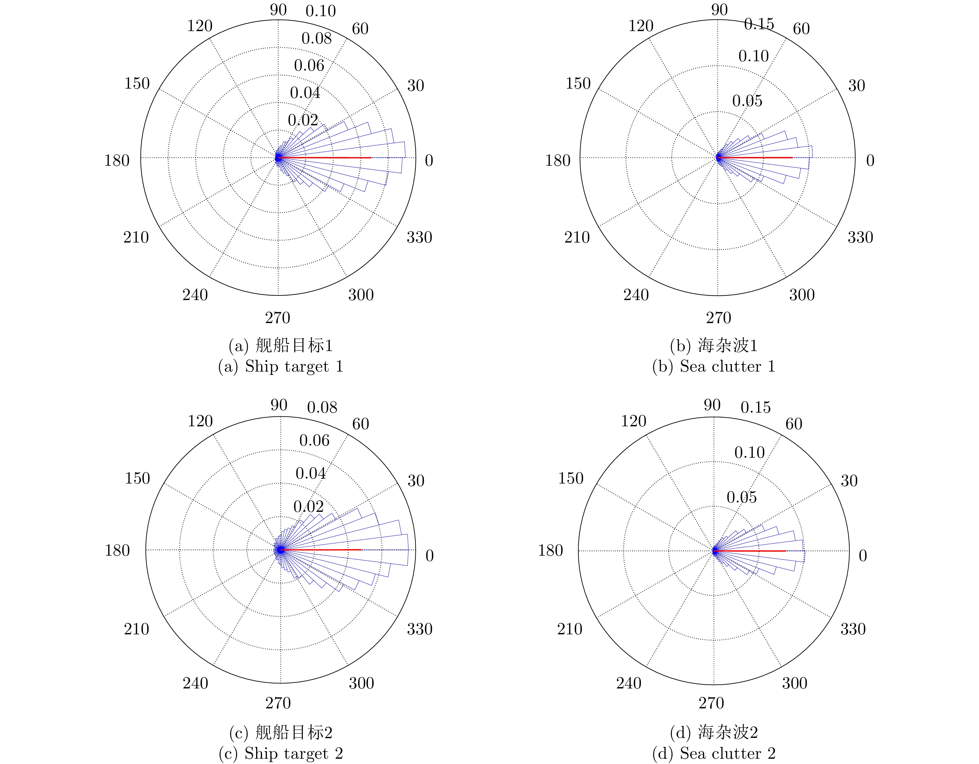
- Figure 3. TerraSAR-X ship target and sea clutter phase histograms (Presented in rose charts. Red line indicates mean direction)
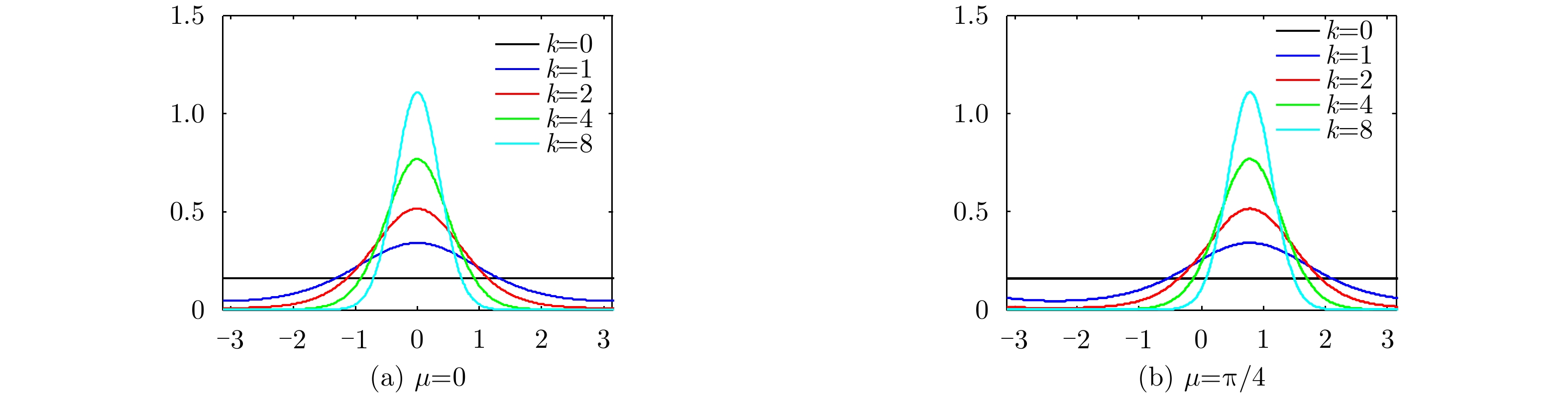
- Figure 4. PDFs for von Mises distribution at different parameters
- Figure 5. TerraSAR-X ship target and sea clutter NPDD images
- Figure 6. TerraSAR-X ship target and sea clutter NPDD histograms (Presented in rose charts. Red line indicates mean direction)
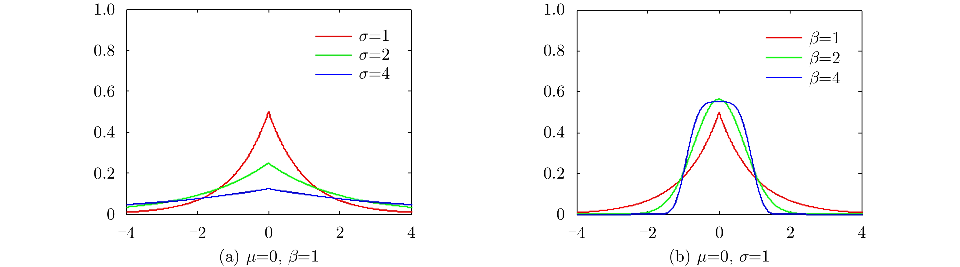
- Figure 7. PDFs for CGGD at different parameters
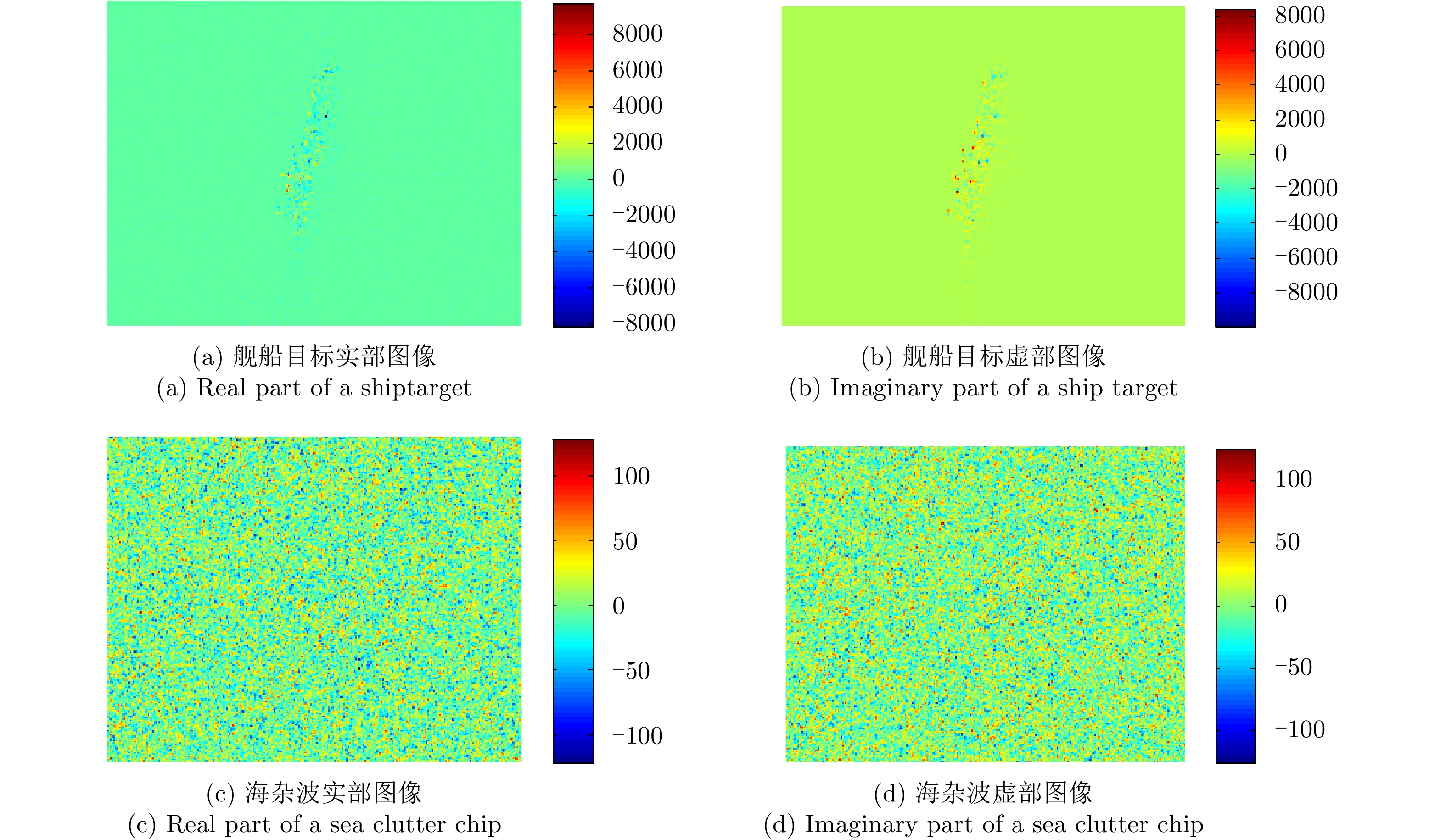
- Figure 8. Real and imaginary parts of ship target and sea clutter images
- Figure 9. Real and imaginary histograms of ship target and sea clutter images
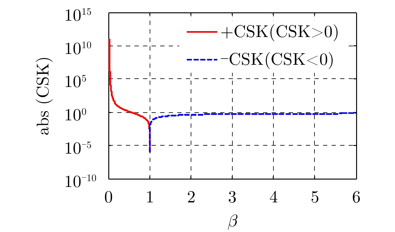
- Figure 10. Relationship between CSK and the shape parameter
- Figure 11. Flowchart of shape parameter estimation of CGGD based on CSK
- Figure 12. MSE results of Novey’s method and our method
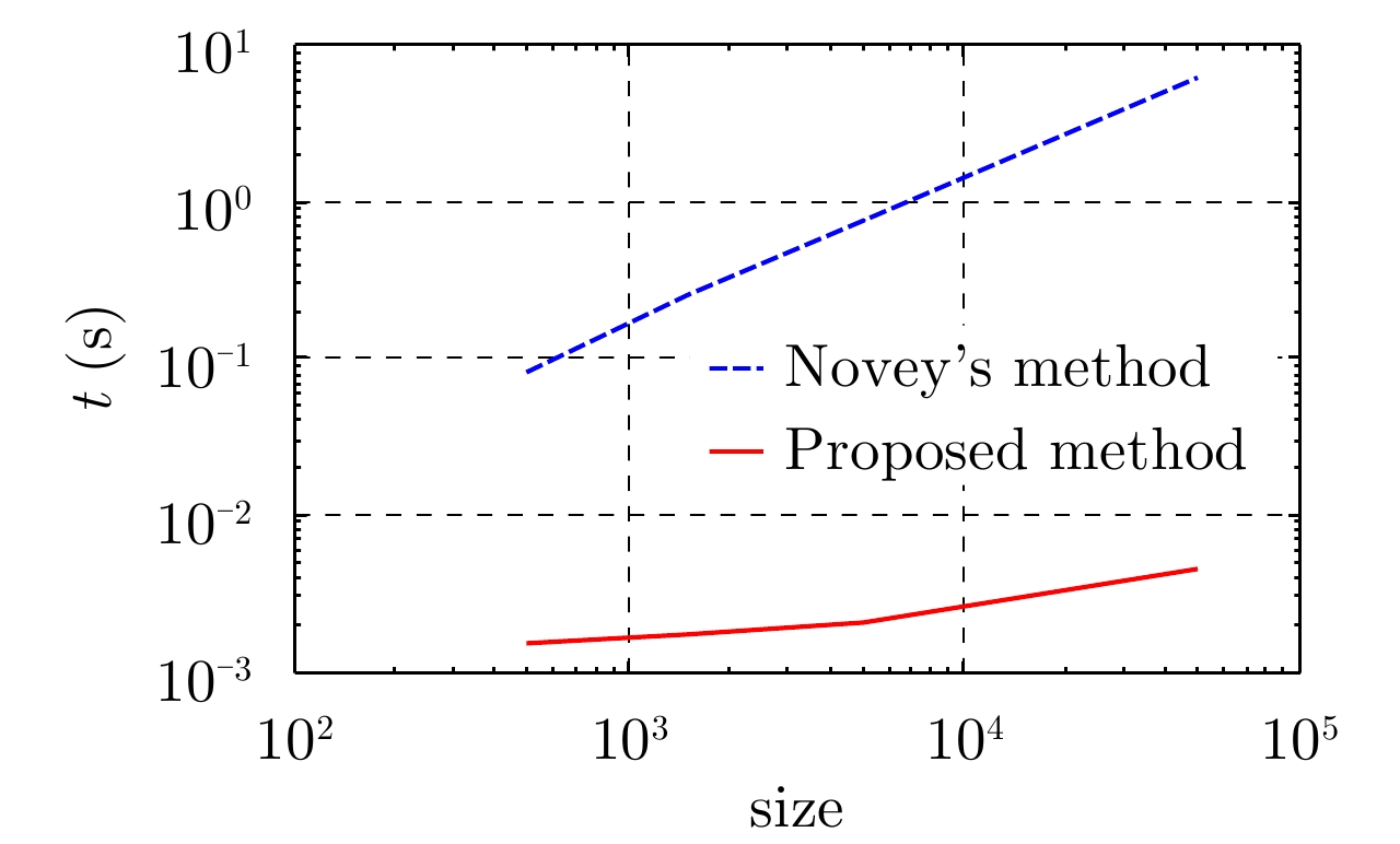
- Figure 13. Average time consumption comparison for a single test of Novey’s method and our method
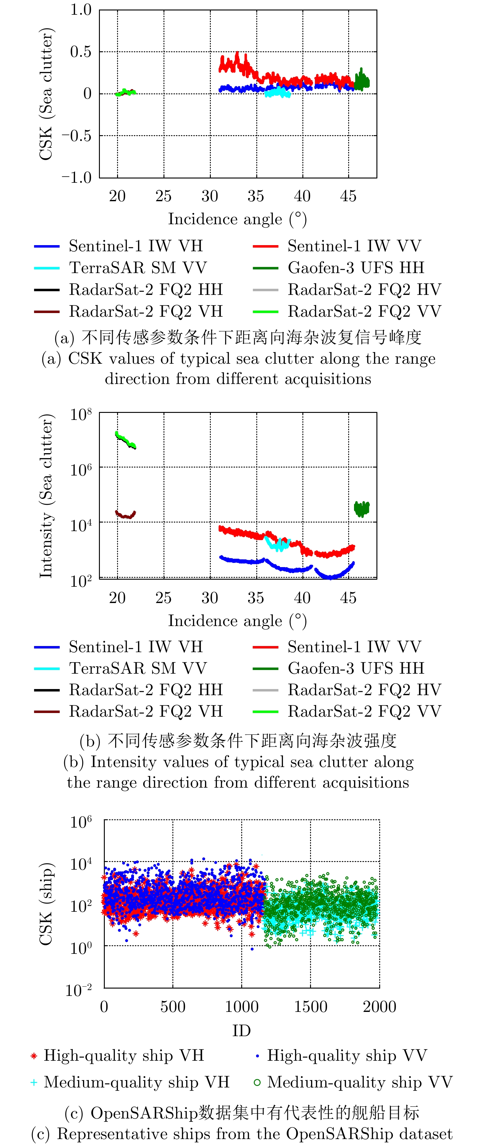
- Figure 14. CSK plots of sea clutter of typical sea clutter and ship targets from different acquisitions
- Figure 15. Ships affected by RFIs in Sentinel-1 images (The green circles represent ships)
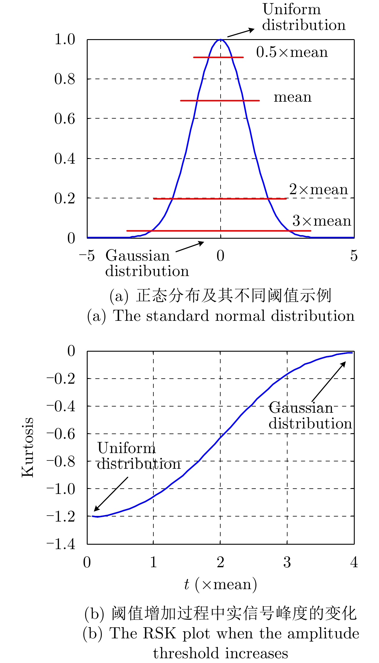
- Figure 16. Illustration of the iteration process for a Gaussian distribution
- Figure 17. Comparison of Otsu and CSK iteration segmentation results