
 Submit Manuscript
 Peer Review
 Editor Work
- Home
- Articles & Issues
-
Data
- Dataset of Radar Detecting Sea
- SAR Dataset
- SARGroundObjectsTypes
- SARMV3D
- AIRSAT Constellation SAR Land Cover Classification Dataset
- 3DRIED
- UWB-HA4D
- LLS-LFMCWR
- FAIR-CSAR
- MSAR
- SDD-SAR
- FUSAR
- SpaceborneSAR3Dimaging
- Sea-land Segmentation
- SAR Multi-domain Ship Detection Dataset
- SAR-Airport
- Hilly and mountainous farmland time-series SAR and ground quadrat dataset
- SAR images for interference detection and suppression
- HP-SAR Evaluation & Analytical Dataset
- GDHuiYan-ATRNet
- Multi-System Maritime Low Observable Target Dataset
- DatasetinthePaper
- DatasetintheCompetition
- Report
- Course
- About
- Publish
- Editorial Board
- Chinese
| Citation: | Ge Jianjun, Li Chunxia. A Dynamic and Adaptive Selection Radar Tracking Method Based on Information Entropy[J]. Journal of Radars, 2017, 6(6): 587-593. doi: 10.12000/JR17081

|
A Dynamic and Adaptive Selection Radar Tracking Method Based on Information Entropy
DOI: 10.12000/JR17081 CSTR: 32380.14.JR17081
-
Abstract
Nowadays, the battlefield environment has become much more complex and variable. This paper presents a quantitative method and lower bound for the amount of target information acquired from multiple radar observations to adaptively and dynamically organize the detection of battlefield resources based on the principle of information entropy. Furthermore, for minimizing the given information entropy’s lower bound for target measurement at every moment, a method to dynamically and adaptively select radars with a high amount of information for target tracking is proposed. The simulation results indicate that the proposed method has higher tracking accuracy than that of tracking without adaptive radar selection based on entropy.
-
Keywords:
- Multi-static radar,
- Information entropy,
- Target tracking
-

-
References
[1] Bar-Shalom Y and Li X R. Multitarget-Multisensor Tracking: Principles and Techniques[M]. Storrs, CT: YBS Publishing, 1995.[2] Koch W. Tracking and Sensor Data Fusion[M]. Berlin, Heidelberg: Springer, 2014.[3] Kalandros M. Covariance control for multisensor systems[J]. IEEE Transactions on Aerospace and Electronic Systems, 2002, 38(4): 1138–1157. DOI: 10.1109/TAES.2002.1145739[4] Yang C, Kaplan L, and Blasch E. Performance measures of covariance and information matrices in resource management for target state estimation[J]. IEEE Transactions on Aerospace and Electronic Systems, 2012, 48(3): 2594–2613. DOI: 10.1109/TAES.2012.6237611[5] Jenkins K L and Castañón D A. Information-based adaptive sensor management for sensor networks[C]. Proceedings of 2011 IEEE American Control Conference, San Francisco, CA, 2011: 4934–4940.[6] Kay S M. Fundamentals of Statistical Signal Processing, Volume I: Estimation Theory[M]. Englewood Cliffs, N. J.: PTR Prentice hall, 1993.[7] Hall D L and McMullen S A H. Mathematical Techniques in Multisensor Data Fusion[M]. Second Edition, Norwood, MA: Artech House, 2004.[8] 李春霞. 宽带雷达空间目标及目标群跟踪方法研究[D]. [博士论文], 北京理工大学, 2015.Li Chun-xia. Research on space target and targets group tracking methods of wideband radar[D]. [Ph.D. dissertation], Beijing Institute of Technology, 2015.[9] Zhang Z T and Zhang J S. A novel strong tracking finite-difference extended Kalman filter for nonlinear eye tracking[J]. Science in China Series F:Information Sciences, 2009, 52(4): 688–694. DOI: 10.1007/s11432-009-0081-1[10] 武勇, 王俊. 混合卡尔曼滤波在外辐射源雷达目标跟踪中的应用[J]. 雷达学报, 2014, 3(6): 652–659. DOI: 10.12000/JR14113Wu Yong and Wang Jun. Application of mixed Kalman filter to passive radar target tracking[J]. Journal of Radars, 2014, 3(6): 652–659. DOI: 10.12000/JR14113[11] Rao B, Xiao S P, and Wang X S. Joint tracking and discrimination of exoatmospheric active decoys using nine-dimensional parameter-augmented EKF[J]. Signal Processing, 2011, 91(10): 2247–2258. DOI: 10.1016/j.sigpro.2011.04.005[12] Liu C Y, Shui P L, and Li S. Unscented extended Kalman filter for target tracking[J]. Journal of Systems Engineering and Electronics, 2011, 22(2): 188–192. DOI: 10.3969/j.issn.1004-4132.2011.02.002[13] Han Y B. A rao-blackwellized particle filter for adaptive beamforming with strong interference[J]. IEEE Transactions on Signal Processing, 2012, 60(6): 2952–2961. DOI: 10.1109/TSP.2012.2189764[14] 李洋漾, 李雯, 易伟, 等. 基于DP-TBD的分布式异步迭代滤波融合算法研究[J]. 雷达学报, 2018, 待出版. DOI: 10.12000/JR17057.Li Yangyang, Li Wen, Yi Wei, et al.. A distributedasynchronous recursive filtering fusion algorithm via DPTBD[J]. Journal of Radars, 2018, accepted. DOI: 10.12000/JR17057. -
Proportional views


- Publishing Ethics
- Journal Insights
- Abstracting & Indexing
- Peer Review Policies
- Guide for Authors
- Conference
- ISSN 2095-283X (Print)ISSN 2097-339X (Online)
- CN 10-1030/TN
- CODEN LXEUAO
About Journal
- Sponsor: China Radio Detection and Ranging Industry Association (CRIA)
- Phone: 010-58887062
- Email:radars@aircas.ac.cn
- Publisher: Leida Xuebao Bianjibu (Editorial office of the Journal of Radars)
Contacts Us

京ICP备20021838号-14
Supported by: Beijing Renhe Information Technology Co. Ltd

Export File
Citation
Format
Content
 DownLoad:


- Figure 1. Radars locations and target trajectory
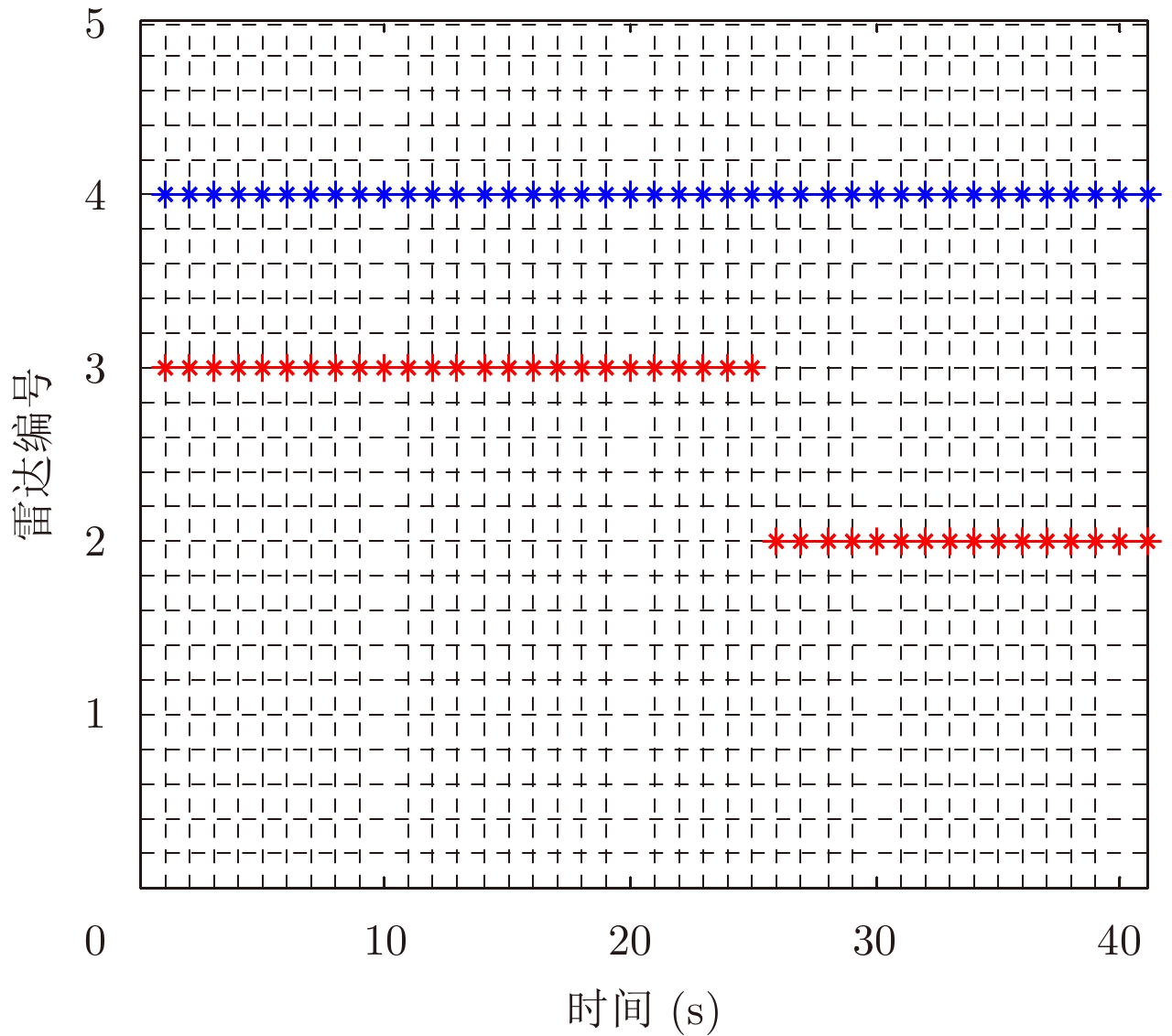
- Figure 2. Radars indexes selected by fusion entropy model
- Figure 3. Comparison of target position RMSE
- Figure 4. Comparison of target velocity RMSE